1. Flow Matching (FM) and Conditional Flow Matching (CFM)

Symbol	Description	Type/Dimension
${𝑝}_0\left(𝑥\right)$	Base distribution (typically simple, e.g., Gaussian)	Probability density
${𝑝}_1\left(𝑥\right)$	Target data distribution	Probability density
${𝑝}_{𝑡}\left(𝑥\right)$	Probability path at time $𝑡$, connecting ${𝑝}_0$ and ${𝑝}_1$	Probability density
${𝑝}_{𝑡}\left(𝑥|𝑧\right)$	Conditional probability path given conditioning variable $𝑧$	Conditional density
$𝑧$	Conditioning variable for constructing conditional flows	Random variable
${𝑢}_{𝑡}\left(𝑥\right)$	Velocity field at time $𝑡$ (marginal)	${ℝ}^{𝑑}$
${𝑢}_{𝑡}\left(𝑥|𝑧\right)$	Conditional velocity field given condition $𝑧$	${ℝ}^{𝑑}$
${𝑢}_{𝑡}^{𝜃}\left(𝑥\right)$	Neural network velocity field with parameters $𝜃$	${ℝ}^{𝑑}$
${𝜓}_{𝑡}\left({𝑥}_0|𝑧\right)$	Conditional flow map from initial point ${𝑥}_0$ to time $𝑡$	${ℝ}^{𝑑}$
$𝑡$	Time variable, typically $𝑡\in \left[0,1\right]$	$ℝ$
$𝑥$	Spatial position variable	${ℝ}^{𝑑}$
${𝑥}_0$	Position at initial time $\left(𝑡=0\right)$	${ℝ}^{𝑑}$
${𝑥}_1$	Position at final time $\left(𝑡=1\right)$	${ℝ}^{𝑑}$
$𝜃$	Neural network parameters	Parameter space
${𝐿}^{\text{CFM}}\left(𝜃\right)$	Conditional Flow Matching loss function	${ℝ}_{+}$
${𝐿}^{\text{FM}}\left(𝜃\right)$	Flow Matching loss function (intractable)	${ℝ}_{+}$

1.1. Flow Matching Overview

Flow Matching is a framework for training continuous normalizing flows by learning velocity fields that transform a simple base distribution into a target data distribution. The key insight is to parameterize the transformation through a time-dependent velocity field ${𝑢}_{𝜃}\left(𝑥,𝑡\right)$ that defines an ordinary differential equation.

Given a probability path ${𝑝}_{𝑡}\left(𝑥\right)$ that interpolates between ${𝑝}_0$ (base distribution) and ${𝑝}_1$ (data distribution), the velocity field must satisfy the continuity equation:

$$\frac{\partial {𝑝}_{𝑡}\left(𝑥\right)}{\partial 𝑡}+\nabla \cdot \left({𝑝}_{𝑡}\left(𝑥\right){𝑢}_{𝜃}\left(𝑥,𝑡\right)\right)=0$$

However, directly learning ${𝑢}_{𝜃}\left(𝑥,𝑡\right)$ from this equation is challenging because:

1. We don't know the true ${𝑝}_{𝑡}\left(𝑥\right)$ for intermediate times
2. The continuity equation provides insufficient supervision
3. There are infinitely many velocity fields satisfying the boundary conditions

CFM solves these issues by introducing conditional probability paths that enable tractable training.

1.2. Conditional Flow Matching (CFM)

The goal of CFM is to find a velocity field ${𝑢}_{𝜃}\left(𝑥,𝑡\right)$. However, there exists an infinite number of velocity fields that can satisfy the continuity equation for a given probability path. In order to get supervision for all $𝑡$, one must fully specify a probability path and its corresponding velocity field.

1.2.1. How to fully specify a probability path ${𝑝}_{𝑡}$ and velocity field ${𝑢}_{𝑡}$?

The key challenge is that solving the continuity equation ${\partial }_{𝑡}{𝑝}_{𝑡}+\nabla \cdot \left({𝑢}_{𝑡}{𝑝}_{𝑡}\right)=0$ for ${𝑢}_{𝑡}$ given ${𝑝}_{𝑡}$ has infinitely many solutions. CFM's core idea is to avoid this difficulty by constructively defining both the probability path and velocity field through:

1. Choose a conditioning variable $𝑧$
2. Design conditional probability paths ${𝑝}_{𝑡}\left(𝑥|𝑧\right)$ with known flow maps ${𝜓}_{𝑡}\left({𝑥}_0|𝑧\right)$
3. Obtain the velocity field analytically via ${𝑢}_{𝑡}\left(𝑥|𝑧\right)={\partial }_{𝑡}{𝜓}_{𝑡}\left({𝑥}_0|𝑧\right)$

We want to ensure two conditions are met:

1. The induced global probability ${𝑝}_{𝑡}\left(𝑥\right)={𝐸}_{𝑧}\left[{𝑝}_{𝑡}\left(𝑥|𝑧\right)\right]$ transforms ${𝑝}_0$ into ${𝑝}_1$.
2. The associated velocity field ${𝑢}_{𝑡}\left(𝑥|𝑧\right)$ has an analytic form obtained from the flow construction.

1.2.2. Linear Interpolation

1.2.2.1. Conditioning on Base and Target Points

The conditional variable $𝑧$ is defined as

$$𝑧\stackrel{\text{ choice }}{=}\left({𝑥}_0,{𝑥}_1\right)\sim {𝑝}_0\times {𝑝}_1$$

1.2.2.2. Flow Construction and Velocity Field

We construct a deterministic linear flow between ${𝑥}_0$ and ${𝑥}_1$:

$${𝜓}_{𝑡}\left({𝑥}_0|𝑧=\left({𝑥}_0,{𝑥}_1\right)\right)\stackrel{\text{ def }}{=}\left(1-𝑡\right)\cdot {𝑥}_0+𝑡\cdot {𝑥}_1$$

This induces the probability path:

$${𝑝}_{𝑡}\left(𝑥|𝑧=\left({𝑥}_0,{𝑥}_1\right)\right)\stackrel{\text{ def }}{=}{𝛿}_{\left(1-𝑡\right)\cdot {𝑥}_0+𝑡\cdot {𝑥}_1}\left(𝑥\right)$$

The velocity field is obtained by differentiating the flow map:

$${𝑢}_{𝑡}\left(𝑥|𝑧=\left({𝑥}_0,{𝑥}_1\right)\right)={\partial }_{𝑡}{𝜓}_{𝑡}\left({𝑥}_0|𝑧\right)={𝑥}_1-{𝑥}_0$$

We can verify that this velocity field satisfies the continuity equation.

1.2.3. Conical Gaussian Paths

1.2.3.1. Alternative Conditioning Choice

We can make other choices for the conditional variable:

$$𝑧\stackrel{\text{ choice }}{=}{𝑥}_1\sim {𝑝}_1$$

1.2.3.2. Flow Construction

We construct a flow that starts from a standard Gaussian and converges to the target point:

$${𝜓}_{𝑡}\left({𝑥}_0|𝑧={𝑥}_1\right)\stackrel{\text{ def }}{=}𝑡{𝑥}_1+\left(1-𝑡\right){𝑥}_0,{𝑥}_0\sim 𝑁\left(0,𝐼\right)$$

This induces the conditional probability path:

$${𝑝}_{𝑡}\left(𝑥|𝑧={𝑥}_1\right)\stackrel{\text{ def }}{=}𝑁\left(𝑡{𝑥}_1,{\left(1-𝑡\right)}^2𝐼𝑑\right)$$

The corresponding velocity field is:

$${𝑢}_{𝑡}\left(𝑥|𝑧={𝑥}_1\right)={\partial }_{𝑡}{𝜓}_{𝑡}\left({𝑥}_0|𝑧\right)=\frac{{𝑥}_1-𝑥}{1-𝑡}$$

where we use the fact that ${𝑥}_0=\frac{𝑥-𝑡{𝑥}_1}{1-𝑡}$ by inverting the flow map.

1.2.4. General construction of conditional probability paths

The general CFM construction follows these steps:

1. First, choose a conditioning variable $𝑧$ (independent of $𝑡$)
2. Second, design flow maps ${𝜓}_{𝑡}\left({𝑥}_0|𝑧\right)$ that connect the source and target distributions
3. Third, obtain conditional probability paths ${𝑝}_{𝑡}\left(𝑥|𝑧\right)$ as the push-forward of the source under the flow
4. Fourth, derive velocity fields ${𝑢}_{𝑡}\left(𝑥|𝑧\right)={\partial }_{𝑡}{𝜓}_{𝑡}\left({𝑥}_0|𝑧\right)$ analytically

The conditional probability paths must satisfy the boundary conditions:

$$\begin{array}{c}\forall 𝑥,{𝐸}_{𝑧}\left[{𝑝}_0\left(𝑥|𝑧\right)\right]={𝑝}_0\left(𝑥\right),\\ \forall 𝑥,{𝐸}_{𝑧}\left[{𝑝}_1\left(𝑥|𝑧\right)\right]={𝑝}_1\left(𝑥\right)\end{array}$$

This construction ensures that:

1. We avoid solving the ill-posed continuity equation
2. The velocity field has an analytical, tractable form
3. The global probability path correctly interpolates between ${𝑝}_0$ and ${𝑝}_1$

1.2.5. From Conditional to Unconditional Velocity

Theorem: Let $𝑧$ be any random variable independent of $𝑡$. Choose conditional probability paths ${𝑝}_{𝑡}\left(𝑥|𝑧\right)$, and let ${𝑢}_{𝑡}\left(𝑥|𝑧\right)$ be the velocity field associated to these paths. Then the marginal velocity field ${𝑢}_{𝑡}\left(𝑥\right)$ associated to the probability path ${𝑝}_{𝑡}\left(𝑥\right)={𝐸}_{𝑧}\left[{𝑝}_{𝑡}\left(𝑥|𝑧\right)\right]$ has a closed-form formula:

$$\forall 𝑡,𝑥,{𝑢}_{𝑡}\left(𝑥\right)={𝐸}_{𝑧|𝑥}\left[{𝑢}_{𝑡}\left(𝑥|𝑧\right)\right]$$

This is intractable in general, so we use a neural network ${𝑢}_{𝑡}^{𝜃}\left(𝑥\right)$ to estimate. The training objective is to minimize the tractable Conditional Flow Matching (CFM) loss:

$${𝐿}^{\text{CFM}}\left(𝜃\right)={𝐸}_{𝑡,𝑧,𝑥}{\Vert {𝑢}_{𝑡}^{𝜃}\left(𝑥\right)-{𝑢}_{𝑡}\left(𝑥|𝑧\right)\Vert }^2$$

We can use the above loss because it's equivalent to directly regressing against the intractable unknown vector field ${𝑢}_{𝑡}\left(𝑥\right)$¹:

$${𝐿}^{\text{CFM}}\left(𝜃\right)={𝐸}_{𝑥,𝑡}{\Vert {𝑢}_{𝑡}^{𝜃}\left(𝑥\right)-{𝑢}_{𝑡}\left(𝑥\right)\Vert }^2+𝐶={𝐿}^{\text{ FM}}\left(𝜃\right)+𝐶$$

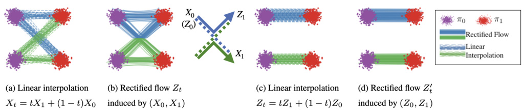
2. Rectified Flow

Rectified Flow is a specific and powerful instantiation of the Flow Matching framework. It simplifies the construction of the probability path and velocity field by focusing on creating the straightest possible trajectories between points from the source and target distributions. This approach not only provides a clear and simple training objective but also leads to highly efficient generative models.

The core idea is to "rectify" the coupling between the base distribution ${𝑝}_0\left(𝑥\right)$ and the target distribution ${𝑝}_1\left(𝑥\right)$. Instead of arbitrary or complex conditional paths, Rectified Flow learns an Ordinary Differential Equation (ODE) that transports mass along straight lines.

2.1. 1-Rectified Flow: The Direct Path

The initial Rectified Flow, often called the 1-rectified flow, is constructed in a manner very similar to the linear interpolation method in CFM.

2.1.1. Construction

We start by creating the simplest possible coupling between the base and target distributions: an independent coupling. We draw a pair of samples, ${𝑥}_0\sim {𝑝}_0\left(𝑥\right)$ and ${𝑥}_1\sim {𝑝}_1\left(𝑥\right)$, and define a straight-line path between them.

The flow map is a direct linear interpolation:

$${𝜓}_{𝑡}\left({𝑥}_0,{𝑥}_1\right)=\left(1-𝑡\right){𝑥}_0+𝑡{𝑥}_1$$

This is the same as the "Linear Interpolation" above. The key difference in Rectified Flow is the focus on this specific construction and its iterative refinement.

The velocity field for this path is constant with respect to time for a given pair $\left({𝑥}_0,{𝑥}_1\right)$:

$${𝑢}_{𝑡}\left(𝑥|𝑧=\left({𝑥}_0,{𝑥}_1\right)\right)={\partial }_{𝑡}{𝜓}_{𝑡}\left({𝑥}_0,{𝑥}_1\right)={𝑥}_1-{𝑥}_0$$

2.1.2. The "Rectified" Velocity Field

While individual paths are straight, the marginal velocity field ${𝑢}_{𝑡}\left(𝑥\right)$ at a point $𝑥$ is the average velocity of all straight-line paths that pass through $𝑥$ at time $𝑡$. This averaging process is what "rectifies" the flow. The resulting marginal velocity field is generally non-linear and complex, and it defines a deterministic flow that transforms ${𝑝}_0$ to ${𝑝}_1$.

The training objective for a neural network ${𝑢}_{𝑡}^{𝜃}\left(𝑥\right)$ is a straightforward regression problem, identical to the CFM loss but with this specific choice of conditional velocity:

$${𝐿}^{\text{RF1}}\left(𝜃\right)={𝐸}_{𝑡,{𝑥}_0,{𝑥}_1}{\Vert {𝑢}_{𝑡}^{𝜃}\left(\left(1-𝑡\right){𝑥}_0+𝑡{𝑥}_1\right)-\left({𝑥}_1-{𝑥}_0\right)\Vert }^2$$

This loss aims to learn the expected velocity $𝐸\left[{𝑥}_1-{𝑥}_0|{𝑥}_{𝑡}=𝑥\right]$ where ${𝑥}_{𝑡}=\left(1-𝑡\right){𝑥}_0+𝑡{𝑥}_1$.

The resulting trained model ${𝑢}_{𝑡}^{𝜃}\left(𝑥\right)$ can then be used to generate samples by solving the ODE $\frac{𝑑{𝑥}_{𝑡}}{𝑑𝑡}={𝑢}_{𝑡}^{𝜃}\left({𝑥}_{𝑡}\right)$ from $𝑡=0$ to $𝑡=1$, starting with a sample ${𝑥}_0\sim {𝑝}_0\left(𝑥\right)$.

2.2. 2-Rectified Flow (and beyond): The "Reflow" Procedure

A key innovation of Rectified Flow is the reflow procedure. While the 1-rectified flow is a significant step, its trajectories are only perfectly straight if the model perfectly learns the conditional expectation. In practice, the generated paths from the 1-rectified flow model will have some curvature.

The reflow procedure aims to iteratively straighten these paths.

2.2.1. The Reflow Algorithm

1. Train the 1-Rectified Flow: First, train a velocity field ${𝑢}_{𝑡}^1\left(𝑥\right)$ using the direct straight-line paths between ${𝑝}_0$ and ${𝑝}_1$ as described above.

2. Generate a New Paired Dataset: Use the trained model ${𝑢}_{𝑡}^1\left(𝑥\right)$ to generate a new set of paired samples.

   • Sample ${𝑧}_0\sim {𝑝}_0\left(𝑥\right)$.
   • Solve the ODE $\frac{𝑑{𝑧}_{𝑡}}{𝑑𝑡}={𝑢}_{𝑡}^1\left({𝑧}_{𝑡}\right)$ from $𝑡=0$ to $𝑡=1$ to obtain the corresponding endpoint ${𝑧}_1$.
   • This creates a new dataset of pairs $\left({𝑧}_0,{𝑧}_1\right)$ that represent a deterministic coupling induced by the 1-rectified flow.

3. Train the 2-Rectified Flow: Train a new velocity field ${𝑢}_{𝑡}^2\left(𝑥\right)$ using the same loss function, but on the new data pairs $\left({𝑧}_0,{𝑧}_1\right)$.

$${𝐿}^{\text{RF2}}\left(𝜃\right)={𝐸}_{𝑡,{𝑧}_0,{𝑧}_1}{\Vert {𝑢}_{𝑡}^{𝜃}\left(\left(1-𝑡\right){𝑧}_0+𝑡{𝑧}_1\right)-\left({𝑧}_1-{𝑧}_0\right)\Vert }^2$$

This process can be repeated to create 3-rectified flows and so on, with each iteration producing increasingly straight trajectories.

References

1. A Visual Dive into Conditional Flow Matching
2. Flow Matching Guide and Code
3. Flow Straight and Fast: Learning to Generate and Transfer Data with Rectified Flow