1. Ordinary Differential Equation (ODE)

An Ordinary Differential Equation (ODE) is a mathematical equation that relates a function with its derivatives. In its simplest form, an ODE can be written as:

where $𝑓\left(𝑡\right)$ is the unknown function we want to find, and $𝑢$ is a known function that describes how $𝑓$ changes with respect to time $𝑡$. The solution to an ODE is a function that satisfies this equation for all values of $𝑡$ in some interval. If we know the initial state $𝑓\left(0\right)$, this problem becomes an initial value problem (IVP).

1.1. Neural ODE networks

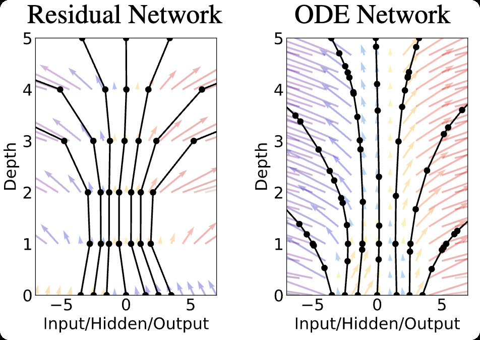
Let's start with a brief introduction to Neural ODE networks. These networks represent a significant advancement in deep learning by modeling continuous-time dynamics using ordinary differential equations. The key insight is that many deep learning architectures can be viewed as discretized versions of continuous transformations.

Traditional models like residual networks, recurrent neural network decoders, and normalizing flows build complex transformations by composing a sequence of transformations to a hidden state:

These iterative updates can be seen as an Euler discretization of a continuous transformation.

What happens as we add more layers and take smaller steps? In the limit, we parameterize the continuous dynamics of hidden units using an ODE specified by a neural network:

The neural network $𝑢$ acts as a vector field that determines how the hidden state evolves over time.

1.2. Velocity Field, Flow and Probability Path

Let's understand these three key concepts in the context of continuous transformations:

1. Velocity Field $𝑢\left(𝑥,𝑡\right)$: This is a vector field that specifies the direction and speed of movement at each point in space and time. It tells us how points are moving through space. In the context of neural networks, this is often parameterized by a neural network that takes the current state and time as input.

2. Flow $𝑓\left(𝑥,𝑡\right)$: The flow represents the actual trajectory or path that points follow under the influence of the velocity field. It's the solution to the ODE defined by the velocity field. Given an initial point ${𝑥}_0$, the flow tells us where that point will be at any time $𝑡$.

3. Probability Path ${𝑝}_{𝑡}$: This represents how the probability distribution evolves over time. As points move according to the flow, the probability mass gets transported along with them. The probability path shows how the initial distribution transforms into the target distribution.

These three concepts are deeply interconnected:

• The velocity field determines the flow through the ODE
• The flow transforms points, which in turn determines how the probability distribution evolves
• The continuity equation ensures that probability mass is conserved during this transformation¹. Under technical conditions and up to divergence-free vector fields, for a given ${𝑝}_{𝑡}$ (resp. $𝑢$) there exists a $𝑢$ (resp. ${𝑝}_{𝑡}$) such that the pair solves the continuity equation.

2. Stochastic Differential Equation (SDE)

See here.

References

1. Neural Ordinary Differential Equations
2. A Visual Dive into Conditional Flow Matching