A primer on GPUs

October 12, 2025

by Leonardo

1. CPU vs GPU: Design Philosophy

1.1. CPU: Latency-Oriented Design

Components:

Arithmetic & Logic Unit (ALU): Execute operations
Control Unit: Decide which operation to execute next
Cache Unit: Cache data for operations to use

Goal: Minimize latency (completion time - start time)

$\to$ Any program can get a speedup for free

Approach: Improve clock rate

But clock rate scaling stopped after 2005 due to power wall

1.2. GPU: Throughput-Oriented Design

Goal: Maximize throughput ( $#$ operations executed per second)

$\to$ Programs get speedup if operations are packed into batches

Approach: More ALUs, less control and less cache

2. CUDA Architecture

CUDA: A parallel computing platform and programming model developed by NVIDIA

CUDA = Compute Unified Device Architecture (but now NVIDIA rarely expands this acronym)
Allows developers to accelerate compute-intensive applications on GPUs using C, C++, and Fortran, etc.

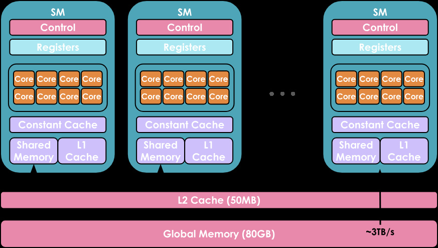
2.1. Hardware Organization

2.1.1. Compute Hierarchy

GPUs have a hierarchical compute organization:

Streaming Multiprocessors (SMs): Array of compute units
CUDA Cores: Individual processors within each SM
Only CUDA cores in the same SM can communicate very efficiently

2.1.2. Memory Hierarchy

From fastest/smallest to slowest/largest:

Registers: Private to each thread
Shared Memory / L1 Cache: Shared by threads in the same SM
L2 Cache: Shared by all SMs
Global Memory: Largest (e.g., 80 GB for H100) but slowest

2.1.3. Terminology

Host = CPU; Device = GPU
Kernel = Code running on GPU, compiled from CUDA/Triton to PTX (Parallel Thread Execution)

2.2. Execution Hierarchy

2.2.1. Thread Level

The smallest execution unit. Each thread executes the same kernel code but processes different data based on its unique thread ID.

2.2.2. Warp Level

32 threads are grouped into a warp.

A warp is the fundamental scheduling unit in NVIDIA GPUs
All threads in a warp execute the same instruction simultaneously (SIMT: Single Instruction, Multiple Thread)
If threads diverge (e.g., due to conditional branches), the warp serializes execution, reducing efficiency
Warps execute independently and can be scheduled in any order

2.2.3. Block Level

Warps are grouped into blocks (also called thread blocks).

Block size is flexible: typically 128, 256, 512, or 1,024 threads (must be a multiple of 32)
Each block is assigned to a single SM and cannot migrate
Threads within a block can:
- Share data via shared memory
- Synchronize using __syncthreads()
- Coordinate through block-level primitives

2.2.4. Grid Level

Blocks are organized into a grid.

A grid represents the entire kernel launch
Can contain thousands or millions of blocks
Blocks are distributed across available SMs
Blocks execute independently (no synchronization between blocks)
Grid dimensions can be 1D, 2D, or 3D for convenience

2.2.5. Execution Flow

You launch a kernel with a grid of blocks
The GPU scheduler assigns blocks to available SMs
Each SM breaks blocks into warps (32 threads each)
Warps are scheduled on cores within the SM
Some blocks may wait if SMs are fully occupied

2.3. Resource Scheduling and Oversubscription

2.3.1. What happens when blocks > SMs?

GPU uses temporal multiplexing: blocks are queued and executed in waves
First wave: as many blocks as can fit on available SMs execute
When a block completes, the next queued block is assigned to that SM
This allows launching millions of blocks on a GPU with only tens of SMs

2.3.2. What happens when threads > CUDA cores?

Each SM has limited CUDA cores (e.g., 64-128 cores per SM)
But each block can have up to 1,024 threads
GPU uses context switching at warp level:
- Multiple warps are resident on the SM simultaneously
- When one warp stalls (e.g., waiting for memory), another warp executes
- This is called warp scheduling and helps hide memory latency
Example: An SM with 64 cores can handle 32+ resident warps (1,024+ threads)
- At any given cycle, only 2 warps (64 threads) are actively executing
- Other warps are either waiting for memory or waiting to be scheduled

If your kernel uses too many resources, fewer blocks can be resident simultaneously, reducing occupancy.

2.4. SPMD Programming Model

Single-Program Multiple-Data: All threads execute the same kernel code, but each thread determines what data to process using built-in variables.

2.4.1. Thread Identification Variables

threadIdx.x ∈ [0, B): Thread's index within its block (0 to block size - 1)
blockIdx.x ∈ [0, G): Block's index within the grid (0 to grid size - 1)
For 2D/3D grids: Also have .y and .z components

2.4.2. Dimension Variables

blockDim.x = B: Size of each block (number of threads per block)
gridDim.x = G: Size of the grid (number of blocks)

2.4.3. Computing Global Thread ID


1
int global_id = blockIdx.x * blockDim.x + threadIdx.x;

This allows each thread to uniquely identify its position and determine which piece of data to process.

2.5. Performance Considerations

2.5.1. Warp Divergence

When threads in a warp take different execution paths (e.g., if-else branches), the warp must execute both paths serially, masking inactive threads. This reduces performance.

2.5.2. Memory Coalescing

For best performance, threads in a warp should access consecutive memory locations. The GPU can combine these into fewer memory transactions.

2.5.3. Occupancy

The ratio of active warps to maximum possible warps on an SM. Higher occupancy helps hide memory latency but requires balancing:

Registers per thread (fewer = more concurrent threads)
Shared memory per block (less = more concurrent blocks)
Threads per block (too few = wasted resources, too many = resource constraints)

3. PyTorch's Abstraction over CUDA

PyTorch provides a high-level interface to GPU computing, hiding most CUDA complexity while delivering excellent performance.

3.1. Built-in Optimized Kernels

PyTorch implements thousands of optimized CUDA kernels:

Matrix multiplications using cuBLAS and cutlass
Convolutions using cuDNN
Activation functions (ReLU, GELU, etc.)
Normalization layers (BatchNorm, LayerNorm)
Attention mechanisms (including FlashAttention)

These kernels are heavily optimized by NVIDIA and PyTorch engineers, typically much faster than custom implementations.

3.2. Tensor Storage with Strides

PyTorch stores tensors using a strided storage format:

Data stored in contiguous 1D array in memory
Stride tuple maps multi-dimensional indices to 1D positions
Example: 2×3 tensor with strides (3, 1) means element [i, j] is at position i * 3 + j

Benefits: Transpose, slice, and reshape can be zero-copy operations (just change strides).

Gotcha: Non-contiguous tensors may harm performance. Use .contiguous() when needed.

3.3. Asynchronous Execution

PyTorch launches CUDA kernels asynchronously:

Kernel launch returns immediately, CPU continues Python execution
Multiple kernels can be queued and pipelined
CPU-GPU data transfer can overlap with computation
Use torch.cuda.synchronize() to wait for GPU completion (e.g., for timing)

3.4. Memory Bottleneck

Modern GPUs have enormous compute but limited memory bandwidth:

A100: 312 TFLOPS (FP16) but only 1.5 TB/s memory bandwidth
Computing is fast, moving data is slow

Arithmetic Intensity = ( $#$ FLOPs) / ( $#$ bytes transferred)

High intensity (matrix multiply): 100+ FLOPs/byte → compute-bound
Low intensity (element-wise ops): < 1 FLOP/byte → memory-bound

Many deep learning operations are memory-bound, not compute-bound.

3.5. Kernel Fusion

Kernel fusion combines multiple operations into a single kernel to reduce memory traffic:

Without fusion: Each operation reads from and writes to global memory
With fusion: Intermediate results stay in registers/shared memory
Benefits: $2 - 10 \times$ speedup for memory-bound ops, fewer kernel launches

3.6. torch.compile for Automatic Optimization

PyTorch 2.0+ includes torch.compile() for automatic optimization:

What it does:

Traces Python code into a computation graph
Applies optimization passes (kernel fusion, dead code elimination, constant folding, layout optimization)
Generates optimized CUDA code using Triton or cuDNN
Caches compiled kernels for reuse

4. Triton: Block-Level GPU Programming

Triton is a Python-based programming language for writing custom GPU kernels with block-level abstractions, making GPU programming more accessible than raw CUDA.

4.1. Key Features

4.1.1. Direct Block-Level Control

Triton allows you to directly control each thread block:

Write code at the block level rather than individual thread level
Block-level parallelism is explicit and programmer-controlled
Automatically handles warp-level details within blocks
Simpler mental model: think in terms of data tiles processed by blocks

4.1.2. PyTorch-like Tensor Operations

Triton provides familiar tensor operation syntax:

Load and store tensors with PyTorch-like operations
Element-wise operations on block-level tiles
Supports masked operations for handling boundaries
Automatic memory coalescing within blocks

4.1.3. Automatic Meta-Parameter Tuning

Triton's compiler automatically optimizes performance-critical parameters:

Block sizes (number of threads per block)
Memory access patterns
Register allocation strategies
Shared memory usage

The @triton.autotune decorator tests multiple configurations and selects the fastest for your hardware.

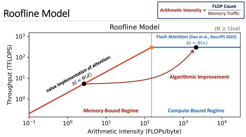
5. Roofline Model: Performance Analysis Framework

The Roofline Model is a conceptual framework for understanding performance bottlenecks in GPU programs. It visualizes whether a kernel is limited by compute capability or memory bandwidth.

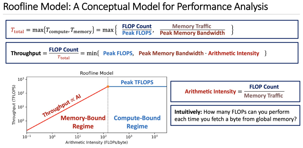
5.1. Key Concepts Explained

5.1.1. Throughput - What Your Kernel Actually Achieves

Definition: The actual computation speed your kernel achieves in practice.

Unit: TFLOPS (Tera FLOPs = trillion floating-point operations per second)

Formula:

Throughput = \frac{FLOP Count}{Execution Time}

Important distinctions:

Peak FLOPS: GPU's maximum theoretical speed (hardware spec, e.g., A100 = 312 TFLOPS)
Achieved Throughput: Your kernel's actual speed (always ≤ Peak FLOPS)

5.1.2. Arithmetic Intensity (AI) - A Property of Your Algorithm

Definition: How much computation you do per byte of data transferred from global memory.

Formula:

AI = \frac{Total FLOPs}{Bytes Transferred from Global Memory}

Unit: FLOPs/byte

Critical insight: AI is a property of your algorithm/kernel, NOT the GPU hardware!

What determines AI:

Algorithm design (what operations you perform)
Data reuse patterns (how many times you use loaded data)
Fusion strategy (combining operations)

5.2. FlashAttention

5.2.1. Standard Self-Attention Mechanism

The standard self-attention mechanism computes:

𝑂 = softmax (𝑄 𝐾^{𝑇}) 𝑉

where $𝑄, 𝐾, 𝑉 \in ℝ^{𝑁 \times 𝑑}$ represent the query, key, and value matrices respectively, with $𝑁$ being the sequence length and $𝑑$ the head dimension.

5.2.1.1. Naive Implementation

A straightforward implementation follows these sequential steps:

Compute the attention scores: $𝑆 = 𝑄 𝐾^{𝑇} \in ℝ^{𝑁 \times 𝑁}$
Apply softmax normalization: $𝑃 = softmax (𝑆) \in ℝ^{𝑁 \times 𝑁}$
Compute the output: $𝑂 = 𝑃 𝑉 \in ℝ^{𝑁 \times 𝑑}$

Time Complexity: The matrix multiplications dominate the computational cost with $𝑂 (𝑁^{2} 𝑑)$ FLOPs.

Memory Complexity: Both intermediate matrices $𝑆$ and $𝑃$ require $𝑂 (𝑁^{2})$ memory, which becomes prohibitive for long sequences.

HBM I/O Complexity: The total number of memory accesses to High Bandwidth Memory (HBM) is $𝑂 (𝑁 𝑑 + 𝑁^{2})$ , comprising:

Reading $𝑄, 𝐾, 𝑉$ : $𝑂 (𝑁 𝑑)$
Writing and reading $𝑆, 𝑃$ : $𝑂 (𝑁^{2})$

5.2.2. The Memory Access Bottleneck

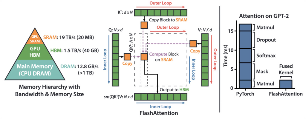
Modern GPUs have a two-tier memory hierarchy:

HBM (High Bandwidth Memory): Large capacity but relatively slow
SRAM (Static Random-Access Memory): Small capacity but extremely fast

The speed difference between SRAM and HBM can be 10 $\times$ or more, making data movement a critical performance bottleneck.

5.2.2.1. The Real Bottleneck: Memory Access Cost (MAC)

Most attention implementations focus solely on minimizing FLOPs, but on modern GPUs, the primary bottleneck is memory bandwidth, not compute.

5.2.2.2. HBM Access Pattern in Standard Attention

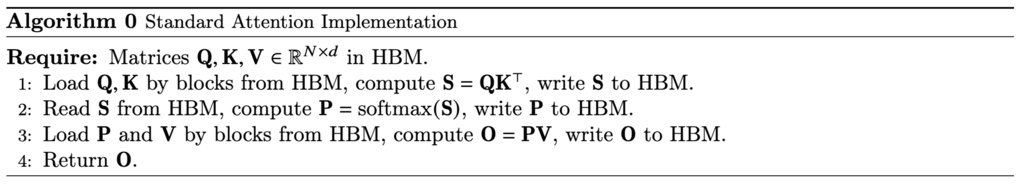
The naive implementation requires 8 HBM read/write operations.

The repeated materialization of large $𝑁 \times 𝑁$ matrices ( $𝑆$ and $𝑃$ ) to HBM is the performance bottleneck.

5.2.3. Flash Attention's Core Idea

5.2.3.1. Trading FLOPs for Memory Access

Flash Attention's key insight is: it's better to recompute values than to access slow HBM. The algorithm:

Reduces HBM accesses by avoiding materialization of the full $𝑁 \times 𝑁$ attention matrices
Uses tiling to keep intermediate results in fast SRAM
Increases FLOPs through recomputation, but achieves overall speedup because memory access is the bottleneck

5.2.3.2. Tiling Strategy

Flash Attention divides the input matrices $𝑄, 𝐾, 𝑉$ into blocks that fit in SRAM:

Load blocks of $𝑄, 𝐾, 𝑉$ into SRAM
Compute attention for these blocks entirely in SRAM
Write only the final output back to HBM

This reduces HBM accesses from $𝑂 (𝑁^{2})$ to $𝑂 (\frac{𝑁^{2}}{𝑀})$ where $𝑀$ is the SRAM size, achieving significant speedup despite performing more FLOPs.

5.2.3.3. The Challenge: Softmax Decomposition

The main technical challenge is: how to compute softmax in a tiled manner?

Standard softmax uses 3-pass safe softmax:

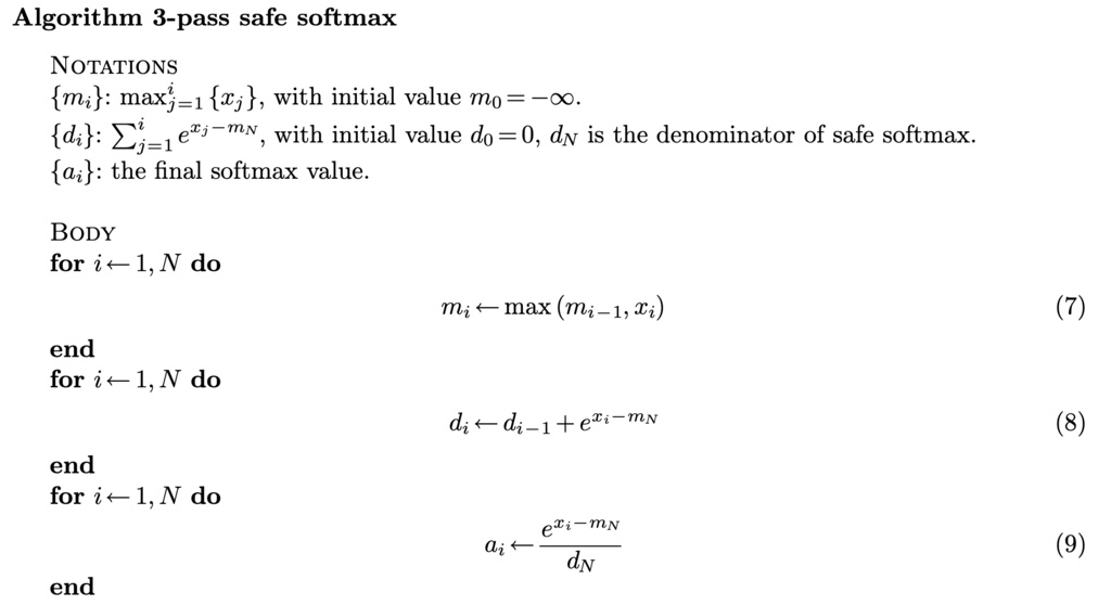
But we actually can use 2-pass online softmax:

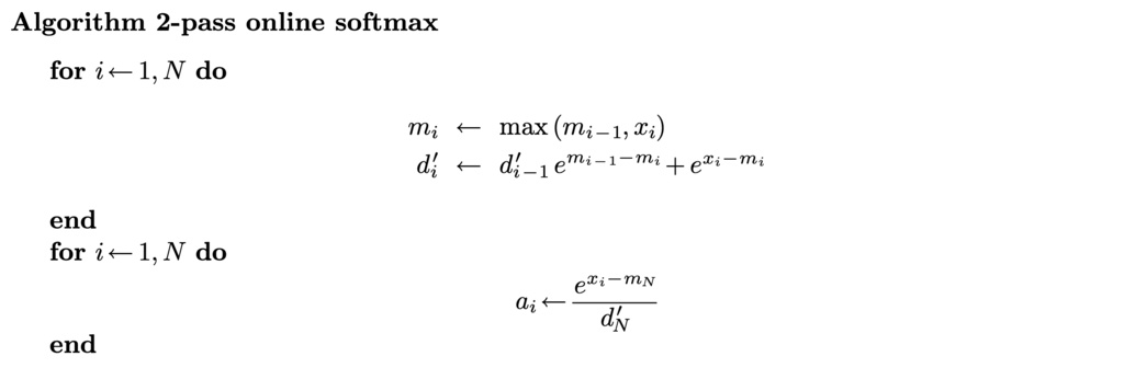
However, it still requires two passes to complete the softmax calculation, can we reduce the number of passes to 1 to minimize global I/O?

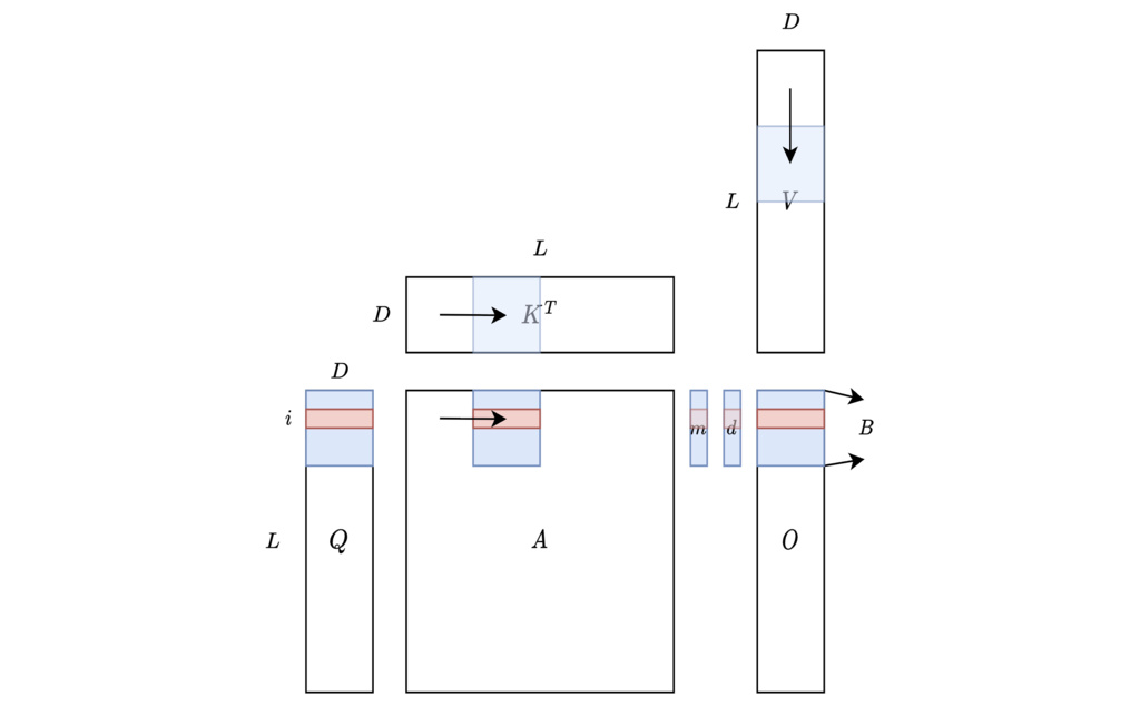
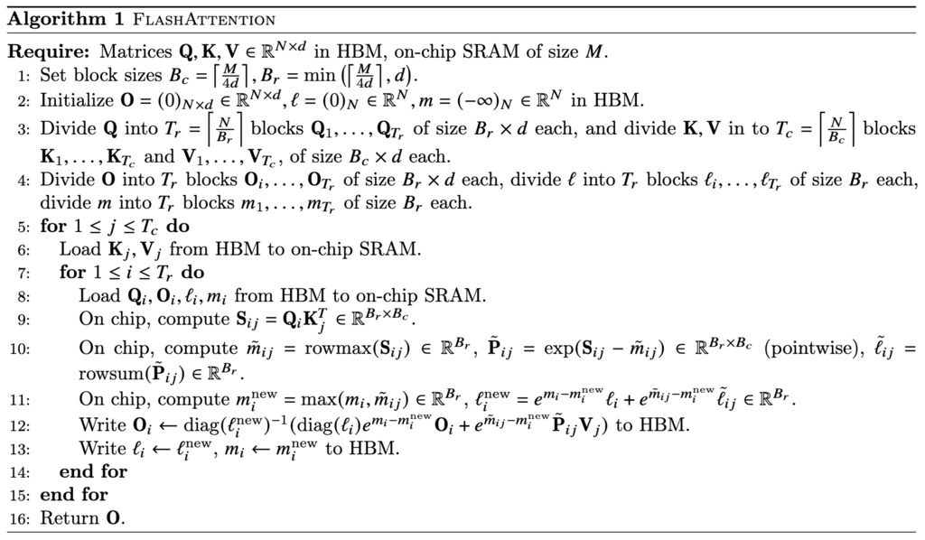
5.2.4. Flash Attention Algorithm

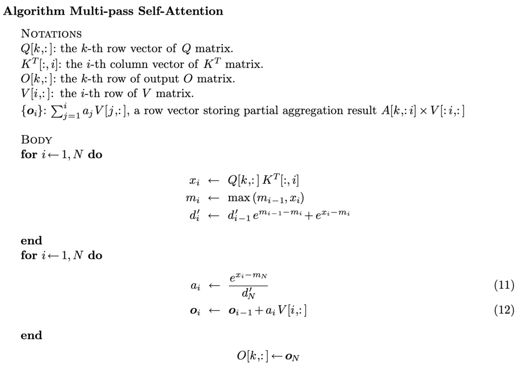
Unfortunately, the answer is "no" for softmax, but in Self-Attention, our final target is not the attention score matrix $𝐴$ , but the $𝑂$ matrix which equals $𝐴 𝑉$ . Can we find a one-pass recurrence form for $𝑂$ instead?

Let's try to formulate the $𝑘$ -th row (the computation of all rows are independent, and we explain the computation of one row for simplicity) of Self-Attention computation as recurrence algorithm:

Using some "surrogate" trick, we can reduce the number of passes to 1:

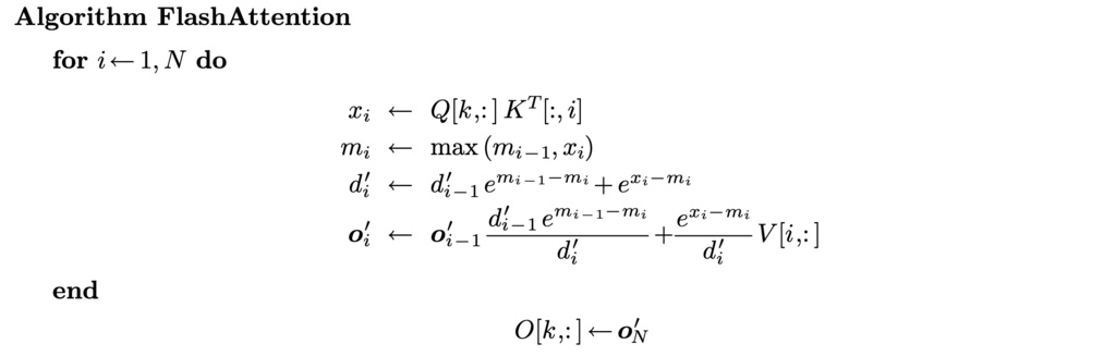
All operations in this algorithm are associative, it is compatible with tiling strategy.

🔒 Access Restricted

Access Control