1. Does Language Training Improve Vision-Language Model Robustness?

A foundational goal of machine learning is to develop models that work reliably across a broad range of data distributions. A central theme of transformer language models is their ability to generalize. By scaling up data and model size, large language models develop emergent abilities that exceed expectations (wei2022emergent). They can also transfer knowledge across domains and tasks (i2024gpt) (brown2020language) (sanh2022multitask). Generalize in length (anil2022exploring) (cai2025extrapolation) and compositional instructions (zhao2024can) (yang2024exploring).

While language models trained on large-scale data tend to be robust to distribution shifts, vision models behave quite differently. Images are inherently noisy and high-dimensional; even small perturbations can push them out-of-distribution, and it's difficult to cover all possible modes. Therefore, improving the robustness of vision models is crucial for their deployment in real-world applications.

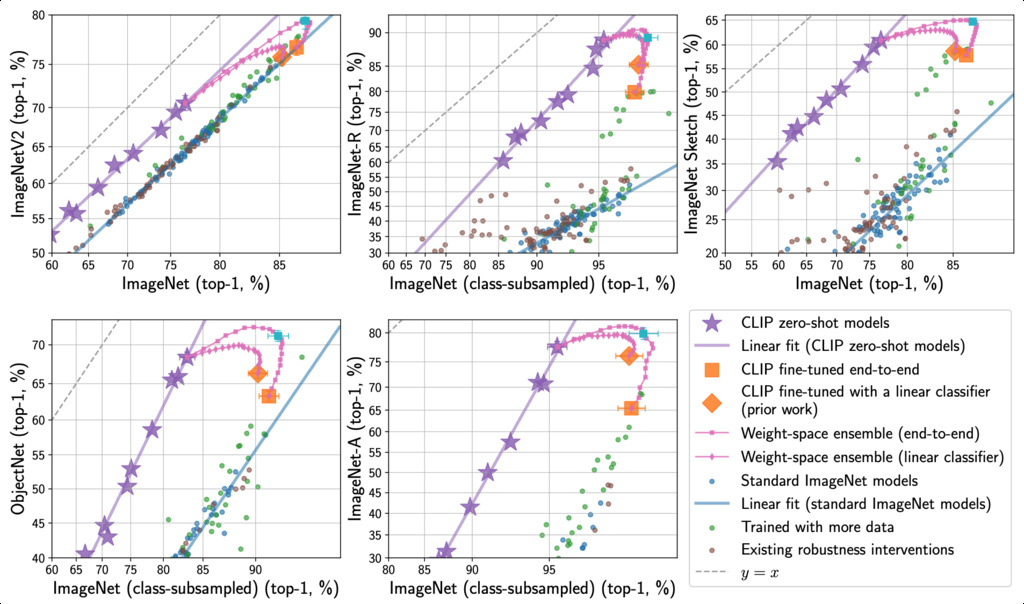
Previous work has demonstrated that CLIP and its variants exhibit greater robustness to distribution shifts compared to standard vision models (wortsman2022robust). This success suggests that pre-training on large, heterogeneous datasets represents a promising direction for increasing robustness (wortsman2022robust) (taori2020measuring). While CLIP is success regard to previous imagenet models, the effectiver robustness cannot surpass the line even with more data and different methods.

Contemporary vision-language models (VLMs) combine pretrained visual encoders with language models, utilizing large-scale datasets for visual instruction tuning (liu2023visual) (liu2023improved) (liu2024llava). These models excel in visual question answering, segmentation, detection, and other multimodal tasks.

Recent work have focused on "vision-centric" VLMs, reducing the reliance and bias on language priors (vo2025vision) (lee2025vl) (wu2025lanp) (leng2024mitigating).

Given the robustness and generalization of Language models and CLIP models, we wonder if such robustness can be transfer to VLMs. We systematically evaluate over 60 VLMs and over 60 visual encoders using carefully constructed multiple-choice classification benchmarks based on ImageNet and its variants.

1.1. Background

To measure robustness, we contrast model accuracy on two related but different distributions, a reference distribution ${𝒟}_{\text{ref}}$ and shifted distribution ${𝒟}_{\text{shift}}$ (wortsman2022robust).¹ We assume both distributions have test sets for evaluation, and ${𝒟}_{\text{ref}}$ has an associated training set ${𝒮}_{\text{ref}}^{\text{tr}}$ which is typically used for training or fine-tuning. The goal for a model is to achieve both high accuracy and consistent performance on the two distributions ${𝒟}_{\text{ref}}$ and ${𝒟}_{\text{shift}}$. This is a natural goal as humans often achieve similar accuracy across the distribution shifts in our study (shankar2020evaluating). For a model $𝑓$, we let ${\text{Acc }}_{\text{ref }}\left(𝑓\right)$ and ${\text{Acc }}_{\text{shift }}\left(𝑓\right)$ refer to classification accuracy on the reference and shifted test sets, respectively.

Following (radford2019language), our focus here is on natural distribution shifts as they are more representative of the real world when no active adversary is present. Specifically, we present our key results for five natural distribution shifts derived from ImageNet (i.e., ${\text{S}}_{\text{ref}}^{\text{tr}}$ is ImageNet):

• ImageNetV2 (IN-V2) (recht2019do), a natural distribution shift derived from ImageNet (IN) (russakovsky2015imagenet) .
• ImageNet-R (IN-R) (hendrycks2021many), renditions (e.g., sculptures, paintings) for 200 ImageNet classes.
• ImageNet Sketch (IN-Sketch) (wang2019learning), which contains sketches instead of natural images.
• ObjectNet (barbu2019objectnet), a test set of objects in various scenes with 113 classes overlapping with ImageNet.
• ImageNet-A (IN-A) (hendrycks2021natural), a test set of natural images misclassified by a ResNet-50 (he2016deep) for 200 ImageNet classes.

To compare the robustness of models with different accuracies on the reference distribution, we follow the effective robustness framework introduced by (miller2021accuracy). Effective robustness quantifies robustness as accuracy beyond a baseline trained only on the reference distribution. A useful tool for studying (effective) robustness are scatter plots that illustrate model performance under distribution shift. These scatter plots display accuracy on the reference distribution on the $𝑥$-axis and accuracy under distribution shift on the $𝑦$-axis, i.e., a model $𝑓$ is shown as a point $\left({\text{Acc }}_{\text{ref }}\left(𝑓\right),{\text{ Acc }}_{\text{ shift }}\left(𝑓\right)\right)$. For the distribution shifts we study, accuracy on the reference distribution is a reliable predictor of accuracy under distribution shift. In other words, there exists a function $𝛽:\left[0,1\right]\to \left[0,1\right]$ such that ${\text{Acc }}_{\text{shift }}\left(𝑓\right)$ approximately equals $𝛽\left({\text{Acc }}_{\text{ref }}\left(𝑓\right)\right)$ for models $𝑓$ trained on the train set ${𝒮}_{\text{ref}}^{\text{tr}}$. Effective robustness (miller2021accuracy) is accuracy beyond this baseline, defined formally as $𝜌\left(𝑓\right)={\text{ Acc }}_{\text{ shift }}\left(𝑓\right)-𝛽\left({\text{Acc }}_{\text{ref }}\left(𝑓\right)\right)$.

In the corresponding scatter plots, effective robustness is vertical movement above expected accuracy under distribution shift. Effective robustness thereby disentangles accuracy changes on the reference distribution from the effect of robustness interventions. When we say that a model is robust to distribution shift, we mean that effective robustness is positive.

1.2. Related Work

(zhang2025out) use in-context learning (ICL) to improve out-of-distribution generalization.

(oh2025understanding) uses information theory to analyze the robustness of VLMs.

(oh2025visual) uses visual instruction bottleneck tuning to improve robustness.

Using RL to improve classification: (liu2025visual) (li2025think)

(li2024exploring) explores how generative mllms perceive more than clip with the same vision encoder.

1.3. Datasets Construction

The original ImageNet validation set is known to have several limitations, including incorrect labels, problematic class definitions, and duplicate or multi-label images (russakovsky2015imagenet) (vasudevan2022when) (northcutt2021pervasive). These issues can lead to an underestimation of true model performance. In response, (kisel2025flaws) consolidated prior label corrections to publish a "clean" label set. We use this label set in our evaluation.

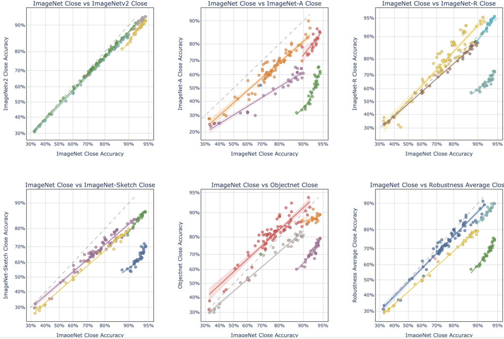
Our evaluation employs a multiple-choice question format. As a baseline, we first constructed a benchmark by randomly sampling distractors. For each image, we created a 5-way multiple-choice question consisting of the ground-truth label and four incorrect labels chosen uniformly at random from the remaining 999 classes. We generated a test set of 5,000 such questions, a sample size sufficient to ensure statistically robust results (see Appendix Section A.3 for an analysis of sample size). However, this random sampling approach proved to be too simplistic; Most models achieve near-saturating accuracy on this task. This finding is consistent with prior work, which has shown that even with 26 random options, model performance remains above 95% (liu2024revisiting).

To create a more challenging and realistic evaluation, we leverage two types of obfuscation:

1. Text obfuscation: We use ImageNet-hierarchy to select distractors that are semantically similar to the ground-truth label, making the classification task harder.
2. Visual obfuscation: We use DION-v3 to select visually confusing distractors.

Although these two approaches generate quite different sets of choices, their results are very similar.

For simplicity, we focus on text obfuscation in the subsequent analysis.

1.4. Results

1. On average, VLMs are more robust than visual encoders since they are more close to $𝑦=𝑥$.
2. Accuracy on the line.
3. For VLMs, SigLip is more robust than CLIP, and web-scale-pretrained ViT is more robust than native training with VLM.

1.4.1. Visual Encoder primarily determine the robustness of VLMs

For VLMs, SigLip is more robust than CLIP, and web-scale-pretrained ViT is more robust than native training with VLM.

1.4.2.

On average, VLMs are more robust than visual encoders since they are more close to $𝑦=𝑥$. But why? Do VLMs learn to use language to improve robustness? Or there's another reason? How can we leverage this to improve its visual encoder's robustness?

We think there are several possible reasons:

1. Language supervision at test time via prompts ❌
2. Large scale pretraining and instruction tunning data ❌
3. The training distribution ❌
4. Language supervision at training time ❌
5. Using Patch tokens instead of cls tokens to encode images
6. Using AnyRes and higher resolutions ❌
7. Generative objectives instead of contrastive objectives ❌

We verified the above reasons one by one.

1.4.3. Language supervision at test time via prompts

To ensure our findings are not artifacts of specific prompting strategies, we evaluate models using five different prompt formulations (detailed in Appendix Section A.4). Figure 3 demonstrates that varying prompt formats does not significantly alter the linear relationship, with all prompting strategies yielding points along the same trend line.

1.4.4. Large scale pretraining and instruction tunning data

1. Small amount of instruction tunning data will arrive at the robustness line (1000 steps)

1.4.5. The training distribution

1. Directly using instruction tunning data to train clip will not help
2. Using CLIP and VLM co-training will not help

1.4.6. Language supervision at training time

1. Initialize LLM and do instruction tunning and some openimages multiple-choice format learning still on VLM robustness line
2. Different LLM have different backbone, but still on the same line

1.4.7. Using Patch tokens instead of cls tokens to encode images

Compressing token might decrease robustness.

Changing Patch tokens to cls tokens will not decrease robustness.

Using patch tokens to do early fusion contrastive learning will not help (yao2022filip) (mukhoti2023open) (zhang2024magiclens)

1.4.8. Using AnyRes and higher resolutions

1. Resize images to 224 $\times$ 224 will decrease score, but still on the robustness line
2. Change LLava-Onevision 'AnyRes' to 'pad' will decrease score, but still on the robustness line
3. Finetuning 224 CLIP with 512 images still on the robustness line.

1.4.9. Generative objectives instead of contrastive objectives

We test VLM2Vec (jiang2024vlm2vec) (meng2025vlm2vec) models and VLM2Vec-LLava trained by (li2024exploring)

After caption pretraining of LLaVA, we fine-tune the VLM2Vec model using LoRA (hu2021lora) on two different datasets. The training is conducted using the LLaVA-1.5-7B model with SigLIP vision encoder as the backbone.

For hyperparameters, we set the learning rate to 2e-5 with a linear scheduler and 0.03 warmup ratio. Training is performed for 400 steps with a batch size of 64 per device using bf16 precision. We apply LoRA with rank $𝑟=4$ to enable efficient fine-tuning while preserving model capacity. The temperature parameter for contrastive learning is set to 0.02, and we use last-token pooling for generating embeddings.

Two training configurations are used: (1) LLaVA finetuning dataset, and (2) CC12M recaption dataset (emporium2024conceptual), which is recaptioned by llama3-llava-next-8b and further cleaned by Meta-Llama-3-8B.

VLM2Vec uses contrastive training to adapt a vision-language model into an embedding model. For VQA dataset, we apply the instruction to the original query $𝑞$ to generate an instruction-conditioned version:

$${𝑞}_{\text{inst }}=\text{ [VISUAL TOKEN] Represent the given image with the following question: {q}}$$

And the target ${𝑡}^{+}$ is the answer to the question. For caption dataset, we only let ${𝑞}_{\text{inst }}=\text{ [VISUAL TOKEN]}$ to achieve similar training strategy as CLIP models. And the target ${𝑡}^{+}$ is the caption of the image.

Given a pretrained VLM, we feed query and target into it to obtain the query and target embeddings (${ℎ}_{{𝑞}_{\text{inst}}}$, ${ℎ}_{{𝑡}^{+}}$) by taking the last layer vector representation of the last token. To train the embedding model, we adopt the standard InfoNCE loss (oord2019representation) $ℒ$ over the in-batch negatives:

$$\min ℒ=-\log \frac{𝜑\left({ℎ}_{{𝑞}_{\text{inst}}},{ℎ}_{{𝑡}^{+}}\right)}{𝜑\left({ℎ}_{{𝑞}_{\text{inst}}},{ℎ}_{{𝑡}^{+}}\right)+\sum _{{𝑡}^{-}\in \mathrm{\mathbb{N}}}𝜑\left({ℎ}_{{𝑞}_{\text{inst}}},{ℎ}_{{𝑡}^{-}}\right)}$$

where $\mathrm{\mathbb{N}}$ is the set of in-batch negatives, and $𝜑\left({ℎ}_{𝑞},{ℎ}_{𝑡}\right)$ is a function that computes the matching score between query $𝑞$ and target $𝑡$. We adopt the temperature-scaled cosine similarity function as $𝜑\left({ℎ}_{𝑞},{ℎ}_{𝑡}\right)=\exp \left(\frac{1}{𝜏}\cos \left({ℎ}_{𝑞},{ℎ}_{𝑡}\right)\right)$, where $𝜏$ is a temperature.

1.4.10. VQA data

Data is one of the deterministic factors in CLIP robustness, different data source might bring different robustness and simply mixing them will not help, quality is more important than quantity (nguyen2022quality).

Overall no pre-training data distribution is consistently the most robust across all evaluation settings.

2. Question-Guided Evidence Selection Explains and Transfers VLM Robustness

2.1. Abstract

We study why, under the same frozen visual encoder, vision-language models (VLMs) exhibit higher effective robustness than CLIP-style models on multiple distribution shifts. We first document a linear “law of robustness” in the probit plane and then give a simple high-dimensional theory showing (i) why models trained with the same frozen features fall on a line, (ii) what sets the line’s slope and which baseline the line passes through, and (iii) why VQA-style task signals raise that line via question-guided evidence selection. Finally, we convert this mechanism into a practical embedding recipe (vlm2vec) that improves OOD performance at matched ID accuracy.

2.2. 1. Introduction

• A paradox: with the visual encoder frozen, why can swapping only the task signal (caption vs VQA) move a model from the “CLIP line-family” up to the “VLM line-family”?
• Observational law: points (ID, OOD) in the probit plane align on lines; towers set line families (height), task signals set slopes and in-line positions.
• Our thesis: VQA acts as question-guided evidence selection over fixed features, rotating the effective decision toward cross-domain stable semantics, which increases slope and lifts the line.
• Contributions: a unified measurement protocol and theory; a mechanism (evidence selection) that explains VLM > CLIP under frozen towers; a deployable embedding recipe (vlm2vec).

We analyze a simple but canonical binary classification example where each training data is parametrized by its ground-truth linear classifier $𝜃\in {𝑅}^{𝑑}$ and its Signal-to-Noise Ratio (SNR) ${𝜌}^2\in {𝑅}_{+}$. Concretely, a training dataset ${𝒟}_{𝑛,𝜃,𝜌}={\left\{\left({𝑥}_{𝑖}\in {𝑅}^{𝑑},{𝑦}_{𝑖}\in \pm 1\right)\right\}}_{𝑖=1}^{𝑛}$ is a set of $𝑛$ i.i.d. paired samples from a joint distribution ${𝑃}_{𝜃,𝜌}$ defined as follows.

Assumption 1 (Data distribution). We define a joint distribution $\left({𝑥}_{𝑖},{𝑦}_{𝑖}\right)\sim {𝑃}_{𝜃,𝜌}$ as (i) ${𝑦}_{𝑖}=\pm 1$ uniformly at random, and (ii) ${𝑥}_{𝑖}={𝑦}_{𝑖}𝜃+\frac{\Vert 𝜃\Vert }{𝜌}{𝑧}_{𝑖}$ where the noise ${𝑧}_{𝑖}$ is zero-mean and has independent entries with variance one. For an observation $\left({𝑥}_{𝑖},{𝑦}_{𝑖}\right)$, we refer to ${\Vert 𝜃\Vert }^2$ as the signal power and $\frac{{\Vert 𝜃\Vert }^2}{{𝜌}^2}$ as the corresponding noise power with SNR ${𝜌}^2$.

Assumption 2 (Trained model distribution). We consider a (random) linear model parameter ${\widehat{𝜃}}_{𝑛,𝜉}\in {𝑅}^{𝑑}$ that predicts a binary label $\text{sign}\left(⟨𝑥,{\widehat{𝜃}}_{𝑛,𝜉}⟩\right)$ for a test example $𝑥\in {𝑅}^{𝑑}$. We assume that the random model ${\widehat{𝜃}}_{𝑛,𝜉}=𝜃+\frac{𝜉\Vert 𝜃\Vert }{𝜌\sqrt{𝑛}}𝑧\in {𝑅}^{𝑑}$, trained on ${𝒟}_{𝑛,𝜃,𝜌}$ is unbiased, $𝐸\left[{\widehat{𝜃}}_{𝑛,𝜉}\right]=𝜃$, and that $𝑧$ has independent entries with variance one each. The randomness comes from the training data as well as any internal randomness in the training algorithm. The parameter $𝜉\in {𝑅}_{+}$ captures the variations in the resulting model distribution due to changes the training algorithm.

Concretely, one canonical example of a trained model is ${\widehat{𝜃}}_{𝑛,𝜉}=\frac{1}{𝑛}{\sum }_{𝑖=1}^{𝑛}{𝑦}_{𝑖}{𝑥}_{𝑖}$. It follows that ${\widehat{𝜃}}_{𝑛}=𝜃+\frac{\Vert 𝜃\Vert }{𝜌\sqrt{𝑛}}𝑧$ with $𝜉=1$. Hence, $𝜉$ measures the randomness of the trained model relative to this simple training algorithm.

We analyze the resulting accuracy when evaluated on two test distributions ${𝑃}_{{𝜃}_1,{𝜌}_1}$ and ${𝑃}_{{𝜃}_2,{𝜌}_2}$ as defined above, with ${\text{Acc }}_{{𝜃}_1,{𝜌}_1}≔{𝑃}_{{𝜃}_1,{𝜌}_1}\left\{\text{sign}\left(⟨𝑋,{\widehat{𝜃}}_{𝑛,𝜉}⟩\right)=𝑌\right\}$, and ${\text{Acc}}_{{𝜃}_2,{𝜌}_2}$ defined similarly. In particular, we are interested in how the accuracy pair $\left({\mathrm{\Phi }}^{-1}\left({\text{Acc}}_{{𝜃}_1,{𝜌}_1}\right),{\mathrm{\Phi }}^{-1}\left({\text{Acc}}_{{𝜃}_2,{𝜌}_2}\right)\right)$ behaves as we vary the sample size $𝑛$ and as we vary the training algorithm represented by $𝜉$. Here, ${\mathrm{\Phi }}^{-1}:\left[0,1\right]\to 𝑅$ is the inverse of the CDF of a standard Gaussian distribution, defined as $\mathrm{\Phi }\left(𝑡\right)=𝑃\left(𝑧<𝑡\right)$ where $𝑧\sim 𝑁\left(0,1\right)$. ${\mathrm{\Phi }}^{-1}$ is also called the probit function. This choice of mapping the accuracy with the probit function is critical in getting the linear relation, which we will explain in Remark 1.

Theorem 1 (Universality of accuracy on the line). Under Assumptions 1 and 2, asymptotically as the dimension $𝑑$ grows linearly in the sample size $𝑛$ such that $\underset{𝑑\to \infty }{\lim }\frac{𝑛}{𝑑}={𝛼}^2$, we have

$$\underset{𝑑\to \infty }{\lim }{\text{ Acc }}_{{𝜃}_1,{𝜌}_1}=\mathrm{\Phi }\left(\cos \left({𝜃}_1,𝜃\right)\frac{{𝜌}_1𝜌𝛼}{𝜉}\right),\text{ and }\underset{𝑑\to \infty }{\lim }{\text{ Acc }}_{{𝜃}_2,{𝜌}_2}=\mathrm{\Phi }\left(\cos \left({𝜃}_2,𝜃\right)\frac{{𝜌}_2𝜌𝛼}{𝜉}\right).$$

Further, under Assumption 5 in the Appendix, for some universal constant $𝑐>0$,

$${\mathrm{\Phi }}^{-1}\left({\text{Acc}}_{{𝜃}_2,{𝜌}_2}\right)=\frac{\cos \left({𝜃}_2,𝜃\right){𝜌}_2}{\cos \left({𝜃}_1,𝜃\right){𝜌}_1}{\mathrm{\Phi }}^{-1}\left({\text{Acc}}_{{𝜃}_1,{𝜌}_1}\right)+𝒪\left(\frac{{𝑒}^{-𝑐𝑛}}{\sqrt{𝑛}}\right).$$

We provide a proof in Appendix F.1. This analysis implies that for any training sample size $𝑛$ and any (variation due to the) training algorithm $𝜉$, the resulting accuracy pair after probit transform lies on a universal line determined by Eq., and the slope only depends on the two test distributions $\left({𝑃}_{{𝜃}_1,{𝜌}_1},{𝑃}_{{𝜃}_2,{𝜌}_2}\right)$ and the training distribution ${𝑃}_{𝜃,𝜌}$. The similarity between the training data and each test dataset is captured by the angles: $\cos \left({𝜃}_1,𝜃\right)$ and $\cos \left({𝜃}_2,𝜃\right)$. More similar training data achieves a larger test accuracy. The hardness of the test distribution is captured by the SNR of each test dataset: ${𝜌}_1$ and ${𝜌}_2$. We emphasize that this line is universal in the sense that the slope does not depend on the sample size $𝑛$ and training algorithm parameter $𝜉$. We are interested in the regime where $𝑛$ scales linearly in $𝑑$ and both are large such that the second term in the above equation is negligible.

Remark 1. Why do we get the accuracy-on-the-line phenomenon? The prediction of the trained (random) linear model on a random test data point $𝑋$ involves the inner product, which performs a natural spatial averaging over the $𝑑$ coordinates. Since the noise across the coordinates is independent and has bounded variance, the central limit theorem applies. The resulting error has a Gaussian tail. Hence, the probit mapping, ${\mathrm{\Phi }}^{-1}\left({\text{Acc}}_{{𝜃}_1,{𝜌}_1}\right)$, is critical in translating accuracy into the relevant mean to standard deviation ratio: $\cos \left({𝜃}_1,𝜃\right){𝜌}_1𝜌\frac{\sqrt{𝑛}}{𝜉\sqrt{𝑑}}$. This is consequently important for getting the universal linear relation, because irrelevant parameters, $𝑛$ and $𝜉$, cancel out in the slope of $\frac{{\mathrm{\Phi }}^{-1}\left({\text{Acc}}_{{𝜃}_2,{𝜌}_2}\right)}{{\mathrm{\Phi }}^{-1}\left({\text{Acc}}_{{𝜃}_1,{𝜌}_1}\right)}$. Refer to the proof of Theorem 1 (Appendix F.1) for more details.

Remark 2. Intersection at the random guess: Previous work that considered models with a wide range of accuracies has found that all lines intersect at a point corresponding to "random guess", which in this binary example is $\left({\mathrm{\Phi }}^{-1}\left(\frac{1}{2}\right),{\mathrm{\Phi }}^{-1}\left(\frac{1}{2}\right)\right)=\left(0,0\right)$. Our theoretical analysis is consistent with this empirical observation: all universal lines intersect at $\left(0,0\right)$ up to a small additive error scaling as $𝒪\left(\frac{1}{\sqrt{𝑛}}\right)$.

3. Proof of Theorem 1

Assumption 5. Under the hypotheses of Theorem 1, suppose there exists a positive constant $𝑐$ such that the third moments are bounded by ${𝐸}_{\left(𝑋,𝑌\right)\sim {𝑃}_{{𝜃}_1,{𝜌}_1}}\left[{\left({𝑋}_{𝑖}𝑌-{𝜃}_{1,𝑖}\right)}^3\right]\le 𝑐{𝐸}_{\left(𝑋,𝑌\right)\sim {𝑃}_{{𝜃}_1,{𝜌}_1}}{\left[{\left({𝑋}_{𝑖}𝑌-{𝜃}_{1,𝑖}\right)}^2\right]}^{\frac{3}{2}}$, ${𝐸}_{\left(𝑋,𝑌\right)\sim {𝑃}_{{𝜃}_2,{𝜌}_2}}\left[{\left({𝑋}_{𝑖}𝑌-{𝜃}_{1,𝑖}\right)}^3\right]\le 𝑐{𝐸}_{\left(𝑋,𝑌\right)\sim {𝑃}_{{𝜃}_2,{𝜌}_2}}{\left[{\left({𝑋}_{𝑖}𝑌-{𝜃}_{1,𝑖}\right)}^2\right]}^{\frac{3}{2}}$, and $𝐸\left[{\left({\widehat{𝜃}}_{𝑛,𝑖}-{𝜃}_{𝑖}\right)}^3\right]\le 𝑐{𝐸\left[{\left({\widehat{𝜃}}_{𝑛,𝑖}-{𝜃}_{𝑖}\right)}^2\right]}^{\frac{3}{2}}$ for all $𝑖\in \left[𝑑\right]$.

Under this assumption, we show that

$$\begin{array}{cc}{\mathrm{\Phi }}^{-1}\left({\text{Acc }}_{{𝜃}_1,{𝜌}_1}\right)& =\cos \left({𝜃}_1,𝜃\right){𝜌}_1\left(\frac{𝜌}{𝜉}\right)\sqrt{\frac{𝑛}{𝑑}}+𝒪\left(\frac{\exp \left({𝜌}_1^2{𝜌}^2\frac{𝑛}{2{𝜉}^2𝑑}\right)}{\sqrt{𝑛}}\right),\text{ and}\end{array}$$$$\begin{array}{cc}{\mathrm{\Phi }}^{-1}\left({\text{Acc }}_{{𝜃}_2,{𝜌}_2}\right)& =\cos \left({𝜃}_2,𝜃\right){𝜌}_2\left(\frac{𝜌}{𝜉}\right)\sqrt{\frac{𝑛}{𝑑}}+𝒪\left(\frac{\exp \left({𝜌}_2^2{𝜌}^2\frac{𝑛}{2{𝜉}^2𝑑}\right)}{\sqrt{𝑛}}\right),\end{array}$$

as it will make the first and second claims straightforward. For $\left({𝑋}_1,{𝑌}_1\right)\sim {𝑃}_{{𝜃}_1,{𝜌}_1}$, the first error event is $\left\{\text{sign}\left(⟨{𝑋}_1,{\widehat{𝜃}}_{𝑛,𝜉}⟩\right)\ne {𝑌}_1\right\}=\left\{⟨{𝑋}_1,{\widehat{𝜃}}_{𝑛,𝜉}⟩{𝑌}_1\le 0\right\}=\left\{⟨𝜃+\left(𝜉\frac{\Vert 𝜃\Vert }{𝜌\sqrt{𝑛}}\right)𝑧,{𝜃}_1+\left(\frac{\Vert {𝜃}_1\Vert }{{𝜌}_1}\right){𝑧}_1⟩\le 0\right\}$, where we used the fact that ${\widehat{𝜃}}_{𝑛,𝜉}=𝜃+\left(𝜉\frac{\Vert 𝜃\Vert }{𝜌\sqrt{𝑛}}\right)𝑧$ and $𝑋𝑌\stackrel{𝑑}{=}{𝜃}_1+\left(\frac{\Vert {𝜃}_1\Vert }{{𝜌}_1}\right){𝑧}_1$. Since the third moments are bounded, applying Berry-Esseen theorem, we get that the probability of error is bounded by $\mathrm{\Phi }\left(-\left(⟨𝜃,{𝜃}_1⟩{𝜌}_1𝜌\frac{\sqrt{𝑛}}{𝜉\Vert {𝜃}_1\Vert \Vert 𝜃\Vert \sqrt{𝑑}}\right)\right)+𝒪\left(\frac{1}{\sqrt{𝑑}}\right)$. This gives ${\text{Acc }}_{{𝜃}_1,{𝜌}_1}=\mathrm{\Phi }\left(⟨𝜃,{𝜃}_1⟩{𝜌}_1𝜌\frac{\sqrt{𝑛}}{𝜉\Vert {𝜃}_1\Vert \Vert 𝜃\Vert \sqrt{𝑑}}\right)+𝒪\left(\frac{1}{\sqrt{𝑑}}\right)$, and consequently

$${\mathrm{\Phi }}^{-1}\left({\text{Acc}}_{{𝜃}_1,{𝜌}_1}\right)=\cos \left({𝜃}_1,𝜃\right){𝜌}_1\left(\frac{𝜌}{𝜉}\right)\sqrt{\frac{𝑛}{𝑑}}+𝒪\left(\frac{{𝑒}^{{\cos \left({𝜃}_1,𝜃\right)}^2{𝜌}_1^2{𝜌}^2\frac{𝑛}{2{𝜉}^2𝑑}}}{\sqrt{𝑛}}\right).$$

This proves the desired claim.

3.1. 2. Measuring on the Probit Line

• Protocol: freeze visual tower $𝜑\left(𝑥\right)$; train heads with different task signals; report $\left({\mathrm{\Phi }}^{-1}\left({\text{Acc}}_{\text{ID}}\right),{\mathrm{\Phi }}^{-1}\left({\text{Acc}}_{\text{OOD}}\right)\right)$ across seeds/compute.
• Definitions: line slope, family height, effective robustness (vertical lift at fixed ID).

3.2. 3. Theory: Why Lines Appear and Who Sets the Slope

3.2.1. 3.1 Setup and Notation

Let $𝜑:{𝑅}^{𝑑}$ be a frozen visual representation. Consider binary one-vs-rest subproblems with labels $𝑌\in \left\{-1,+1\right\}$ and features $𝑋=𝜑(⊷)$. A linear head $𝑤\in {𝑅}^{𝑑}$ predicts by the score $𝑠\left(𝑥\right)=⟨𝑤,𝑋⟩$. Training uses a task signal–induced data distribution ${𝑃}_{\mathrm{tr}}$.

We model class-conditional features by a standard high-dimensional Gaussian location model:

$$𝑋|𝑌=𝑌𝜃+\left(\frac{\Vert 𝜃\Vert }{𝜌}\right)𝑍,𝑍\sim 𝑁\left(0,{𝐼}_{𝑑}\right),$$

where $𝜃\in {𝑅}^{𝑑}$ encodes the task-aligned mean direction under ${𝑃}_{\mathrm{tr}}$, and $𝜌>0$ is an SNR. For evaluation, we have two test distributions with parameters $\left({𝜃}_{\text{ID}},{𝜌}_{\text{ ID}}\right)$ and $\left({𝜃}_{\text{OOD}},{𝜌}_{\text{ OOD}}\right)$.

Define the training direction

$${𝜃}_{\mathrm{tr}}≔{𝐸}_{\left\{\left(𝑋,𝑌\right)\sim {𝑃}_{\mathrm{tr}}\right\}}\left[𝑌𝑋\right].$$

3.2.2. 3.2 Probit-Linearity under Frozen Features

Theorem 1 (Probit linearity). Fix the frozen $𝜑$ and the training distribution ${𝑃}_{\mathrm{tr}}$. Let $ℳ$ be any family of heads $𝑤$ obtained by training on ${𝑃}_{\mathrm{tr}}$ under varying sample sizes, seeds, or regularization, while keeping $𝜑$ fixed. In the high-dimensional regime (with $𝑛,𝑑\text{ to }\infty$ and $\frac{𝑛}{𝑑}\text{ to }{𝛼}^2$), the pair of probit accuracies on two test distributions satisfies, for all $𝑤\in ℳ$,

$${\mathrm{\Phi }}^{-1}\left({\text{Acc }}_{\text{OOD }}\left(𝑤\right)\right)=𝑆\left({𝑃}_{\mathrm{tr}};\text{ ID},\text{ OOD}\right)\cdot {\mathrm{\Phi }}^{-1}\left({\text{Acc }}_{\text{ID }}\left(𝑤\right)\right)+𝜀,$$

where the slope

$$𝑆\left({𝑃}_{\mathrm{tr}};\text{ ID},\text{ OOD}\right)=\frac{\cos \left({𝜃}_{\text{OOD}},{𝜃}_{\mathrm{tr}}\right){𝜌}_{\text{ OOD}}}{\cos \left({𝜃}_{\text{ID}},{𝜃}_{\mathrm{tr}}\right){𝜌}_{\text{ ID}}},$$

the remainder $𝜀$ is negligible in the limit.

Interpretation. All models trained with the same frozen features and the same ${𝑃}_{\mathrm{tr}}$ lie (up to vanishing error) on a common line in the probit plane. The line’s slope depends only on geometric alignment between the training direction and each test direction, modulated by their SNRs, not on sample size or optimizer noise.

Sketch of proof. (i) Under the Gaussian location model, the signed margins ${𝑀}_{𝑖}≔𝑌⟨𝑤,𝑋⟩$ are approximately Gaussian by high-dimensional CLT; misclassification events are tail events controlled by standardized means. (ii) Training on ${𝑃}_{\mathrm{tr}}$ makes $𝑤$ concentrate around the task direction ${𝜃}_{\mathrm{tr}}$ up to a random scale and small orthogonal noise, so $\cos \left({𝜃}_{𝑖},𝑤\right)\approx \cos \left({𝜃}_{𝑖},{𝜃}_{\mathrm{tr}}\right)$. (iii) Probit accuracy ${\mathrm{\Phi }}^{\left\{-1\right\}}\left({\text{Acc}}_{𝑖}\right)$ is asymptotically proportional to $\cos \left({𝜃}_{𝑖},𝑤\right){𝜌}_{𝑖}$ with a common $𝑤$-dependent scale that cancels in the ratio across $𝑖\in \left\{\text{ID},\text{ OOD}\right\}$, yielding a line with slope $𝑆\left({𝑃}_{\mathrm{tr}};\text{ ID},\text{ OOD}\right)$.

Corollary 1 (Which baseline the line passes through). If a baseline head ${𝑤}_{𝐴}$ was trained on the same frozen $𝜑$ and the same ${𝑃}_{\mathrm{tr}}$ (e.g., a CLIP head aligned to web captions on that tower), then its probit point lies on the same line. Consequently, any re-trained heads on ${𝑃}_{\mathrm{tr}}$ (different seeds/strength) will form a line through A. Replacing the tower changes $𝜑$ and typically changes ${𝑃}_{\mathrm{tr}}$’s induced ${𝜃}_{\mathrm{tr}}$, so the family becomes a distinct line that passes through the new baseline (e.g., “through B”).

Corollary 2 (Towers set line families). Changing the visual tower $𝜑$ changes the induced feature geometry and hence the achievable ${𝜃}_{\mathrm{tr}}$ for any given task signal, shifting the family height (the locus of lines you can realize). Empirically, stronger towers (e.g., SigLIP) realize higher families for both CLIP-style and VLM-style training.

3.2.3. 3.3 From Slope to VLM Robustness: Why VQA Lifts the Line

We now link the slope $𝑆\left({𝑃}_{\mathrm{tr}};\text{ ID},\text{ OOD}\right)$ to task signals.

Definition (Question-guided evidence selection). A task signal $𝒯$ (e.g., VQA) induces training reweighting or constraints that increase the alignment between ${𝜃}_{\mathrm{tr}}$ and cross-domain stable evidence while reducing reliance on spurious background factors, all over the same frozen $𝜑$.

Proposition 2 (Task signals that improve cross-domain alignment increase slope). Let ${𝑃}_{\mathrm{tr}}^{\left\{\text{cap}\right\}}$ be a caption-style training distribution and ${𝑃}_{\mathrm{tr}}^{\left\{\text{vqa}\right\}}$ be its VQA-style counterpart on the same $𝜑$. Suppose

$$\frac{\cos \left({𝜃}_{\text{OOD}},{𝜃}_{\mathrm{tr}}^{\left\{\text{vqa}\right\}}\right)}{\cos \left({𝜃}_{\text{ID}},{𝜃}_{\mathrm{tr}}^{\left\{\text{vqa}\right\}}\right)}>\frac{\cos \left({𝜃}_{\text{OOD}},{𝜃}_{\mathrm{tr}}^{\left\{\text{cap}\right\}}\right)}{\cos \left({𝜃}_{\text{ID}},{𝜃}_{\mathrm{tr}}^{\left\{\text{cap}\right\}}\right)},>\frac{\cos \left({𝜃}_{\text{OOD}},{𝜃}_{\mathrm{tr}}^{\left\{\text{cap}\right\}}\right)}{\cos \left({𝜃}_{\text{ID}},{𝜃}_{\mathrm{tr}}^{\left\{\text{cap}\right\}}\right)}.$$

Then

$$𝑆\left({𝑃}_{\mathrm{tr}}^{\left\{\text{vqa}\right\}};\text{ ID},\text{ OOD}\right)>𝑆\left({𝑃}_{\mathrm{tr}}^{\left\{\text{cap}\right\}};\text{ ID},\text{ OOD}\right).$$

Hence, at matched ${\mathrm{\Phi }}^{\left\{-1\right\}}\left({\text{Acc}}_{\text{ID}}\right)$, VQA-trained heads achieve higher ${\mathrm{\Phi }}^{\left\{-1\right\}}\left({\text{Acc}}_{\text{OOD}}\right)$—the line lifts.

Proof (one line). Directly compare the definitions of $𝑆$ for the two training distributions; ${𝜌}_{𝑖}$ cancel in the ratio if unchanged, and the stated inequality on cosine ratios yields the strict ordering of slopes.

Operational takeaway.

• Caption signals that mirror the tower's pretraining web distribution tend to produce ${𝜃}_{\mathrm{tr}}$ nearly collinear with the CLIP baseline direction, so the line passes through the baseline and has a “caption slope”.
• VQA signals impose question-conditioned constraints that select semantically relevant, stable evidence (even with a CLS head), rotating ${𝜃}_{\mathrm{tr}}$ toward directions better shared by ID and OOD. This strictly increases slope and lifts the line—explaining why VLM lines sit above CLIP lines under the same frozen tower.

3.3. 4. What Sets the Family vs What Sets the Slope (Empirics)

• Towers set line families (height): CLIP vs SigLIP.
• Task signals set slopes and on-line positions: caption → baseline line; VQA → higher slope and lift; caption↔VQA mixtures interpolate the slope.

3.4. 5. From Mechanism to Method: A Robust Embedding (vlm2vec)

• Train with question-guided task signals on the frozen tower; distill to a deployable embedding.
• Observation: vlm2vec (VQA) lies on the VLM family; vlm2vec (caption) lies on the CLIP family.

3.5. 6. Negative Results (Concise)

• Prompt templates, resolution, and generative vs discriminative objectives: second-order effects on the line; do not change the family and rarely change the slope materially under frozen towers.

3.6. 7. Discussion and Future Work

• Patch tokens as an amplifier of evidence selection (left to future mechanistic analysis).
• Data efficiency and compute–robustness tradeoffs; failure modes and biases.

References

References

1. Anil, C., Wu, Y., Andreassen, A., Lewkowycz, A., Misra, V., Ramasesh, V., Slone, A., Gur-Ari, G., Dyer, E., and Neyshabur, B. Exploring Length Generalization in Large Language Models. Advances in Neural Information Processing Systems (Neurips), 2022.
2. Barbu, A., Mayo, D., Alverio, J., Luo, W., Wang, C., Gutfreund, D., Tenenbaum, J., and Katz, B. Objectnet: A large-scale bias-controlled dataset for pushing the limits of object recognition models. Advances in Neural Information Processing Systems (Neurips), 2019.
3. Brown, T., Mann, B., Ryder, N., Subbiah, M., Kaplan, J. D., Dhariwal, P., Neelakantan, A., Shyam, P., Sastry, G., Askell, A., Agarwal, S., Herbert-Voss, A., Krueger, G., Henighan, T., Child, R., Ramesh, A., Ziegler, D., Wu, J., Winter, C., … Amodei, D. Language Models are Few-Shot Learners. Advances in Neural Information Processing Systems (Neurips), 2020.
4. Cai, Y., Yin, F., Hammou, D., and Mantiuk, R. Do computer vision foundation models learn the low-level characteristics of the human visual system?. IEEE/CVF Conference on Computer Vision and Pattern Recognition (CVPR), 2025.
5. Cai, Z., Lee, N., Schwarzschild, A., Oymak, S., and Papailiopoulos, D. Extrapolation by Association: Length Generalization Transfer in Transformers, 2025.
6. Emporium, C. conceptual-captions-cc12m-llavanext, 2024.
7. He, K., Zhang, X., Ren, S., and Sun, J. Deep residual learning for image recognition. IEEE/CVF Conference on Computer Vision and Pattern Recognition (CVPR), 2016.
8. Hendrycks, D., Basart, S., Mu, N., Kadavath, S., Wang, F., Dorundo, E., Desai, R., Zhu, T., Parajuli, S., Guo, M., and others. The many faces of robustness: A critical analysis of out-of-distribution generalization. IEEE/CVF Conference on Computer Vision and Pattern Recognition (CVPR), 2021.
9. Hendrycks, D., Zhao, K., Basart, S., Steinhardt, J., and Song, D. Natural adversarial examples. IEEE/CVF Conference on Computer Vision and Pattern Recognition (CVPR), 2021.
10. Hu, J. E., Shen, Y., Wallis, P., Allen-Zhu, Z., Li, Y., Wang, S., and Chen, W. LoRA: Low-Rank Adaptation of Large Language Models. International Conference on Learning Representations (ICLR), 2021.
11. Huh, M., Cheung, B., Wang, T., and Isola, P. The Platonic Representation Hypothesis. International Conference on Machine Learning (ICML), 2024.
12. OpenAI, Achiam, J., Adler, S., Agarwal, S., Ahmad, L., Akkaya, I., Aleman, F. L., Almeida, D., Altenschmidt, J., Altman, S., Anadkat, S., Avila, R., Babuschkin, I., Balaji, S., Balcom, V., Baltescu, P., Bao, H., Bavarian, M., Belgum, J., … Zoph, B. GPT-4 Technical Report, 2024.
13. Jiang, Z., Meng, R., Yang, X., Yavuz, S., Zhou, Y., and Chen, W. VLM2Vec: Training Vision-Language Models for Massive Multimodal Embedding Tasks. International Conference on Learning Representations (ICLR), 2024.
14. Kisel, N., Volkov, I., Hanzelková, K., Janouskova, K., and Matas, J. Flaws of ImageNet, Computer Vision's Favorite Dataset. ICLR Blogposts, 2025.
15. Lee, K.-i., Kim, M., Yoon, S., Kim, M., Lee, D., Koh, H., and Jung, K. VLind-Bench: Measuring Language Priors in Large Vision-Language Models. Proceedings of the Annual Conference of the Nations of the Americas Chapter of the Association for Computational Linguistics (NAACL), 2025.
16. Leng, S., Zhang, H., Chen, G., Li, X., Lu, S., Miao, C., and Bing, L. Mitigating Object Hallucinations in Large Vision-Language Models through Visual Contrastive Decoding. IEEE/CVF Conference on Computer Vision and Pattern Recognition (CVPR), 2024.
17. Li, S., Koh, P. W., and Du, S. S. Exploring how generative mllms perceive more than clip with the same vision encoder. Proceedings of the Annual Meeting of the Association for Computational Linguistics (ACL), 2024.
18. Li, M., Zhong, J., Zhao, S., Lai, Y., Zhang, H., Zhu, W. B., and Zhang, K. Think or Not Think: A Study of Explicit Thinking in Rule-Based Visual Reinforcement Fine-Tuning, 2025.
19. Liu, H., Li, C., Li, Y., and Lee, Y. J. Improved Baselines with Visual Instruction Tuning. IEEE/CVF Conference on Computer Vision and Pattern Recognition (CVPR), 2023.
20. Liu, H., Li, C., Wu, Q., and Lee, Y. J. Visual Instruction Tuning. Advances in Neural Information Processing Systems (Neurips), 2023.
21. Liu, H., Li, C., Li, Y., Li, B., Zhang, Y., Shen, S., and Lee, Y. J. LLaVA-NeXT: Improved reasoning, OCR, and world knowledge, 2024.
22. Liu, H., Xiao, L., Liu, J., Li, X., Feng, Z., Yang, S., and Wang, J. Revisiting MLLMs: An In-Depth Analysis of Image Classification Abilities, 2024.
23. Liu, Z., Sun, Z., Zang, Y., Dong, X., Cao, Y., Duan, H., Lin, D., and Wang, J. Visual-RFT: Visual Reinforcement Fine-Tuning. IEEE/CVF International Conference on Computer Vision (ICCV), 2025.
24. Meng, R., Jiang, Z., Liu, Y., Su, M., Yang, X., Fu, Y., Qin, C., Chen, Z., Xu, R., Xiong, C., Zhou, Y., Chen, W., and Yavuz, S. VLM2Vec-V2: Advancing Multimodal Embedding for Videos, Images, and Visual Documents, 2025.
25. Miller, J. P., Taori, R., Raghunathan, A., Sagawa, S., Koh, P. W., Shankar, V., Liang, P., Carmon, Y., and Schmidt, L. Accuracy on the Line: on the Strong Correlation Between Out-of-Distribution and In-Distribution Generalization. International Conference on Machine Learning (ICML), 2021.
26. Mukhoti, J., Lin, T.-Y., Poursaeed, O., Wang, R., Shah, A., Torr, P. H., and Lim, S.-N. Open vocabulary semantic segmentation with patch aligned contrastive learning. IEEE/CVF Conference on Computer Vision and Pattern Recognition (CVPR), 2023.
27. Nguyen, T., Ilharco, G., Wortsman, M., Oh, S., and Schmidt, L. Quality Not Quantity: On the Interaction between Dataset Design and Robustness of CLIP. Advances in Neural Information Processing Systems (Neurips), 2022.
28. Northcutt, C. G., Athalye, A., and Mueller, J. W. Pervasive Label Errors in Test Sets Destabilize Machine Learning Benchmarks. Neural Information Processing Systems: Datasets and Benchmarks Track, 2021.
29. Oh, C., Fang, Z., Im, S., Du, X., and Li, Y. Understanding Multimodal LLMs Under Distribution Shifts: An Information-Theoretic Approach. International Conference on Machine Learning (ICML), 2025.
30. Oh, C., Li, J., Im, S., and Li, Y. Visual Instruction Bottleneck Tuning, 2025.
31. Oord, A. van den, Li, Y., and Vinyals, O. Representation Learning with Contrastive Predictive Coding, 2019.
32. Radford, A., Wu, J., Child, R., Luan, D., Amodei, D., Sutskever, I., and others. Language models are unsupervised multitask learners, 2019.
33. Recht, B., Roelofs, R., Schmidt, L., and Shankar, V. Do ImageNet Classifiers Generalize to ImageNet?. International Conference on Machine Learning (ICML), 2019.
34. Russakovsky, O., Deng, J., Su, H., Krause, J., Satheesh, S., Ma, S., Huang, Z., Karpathy, A., Khosla, A., Bernstein, M., and others. Imagenet large scale visual recognition challenge. International Journal of Computer Vision (IJCV), 2015.
35. Sanh, V., Webson, A., Raffel, C., Bach, S. H., Sutawika, L., Alyafeai, Z., Chaffin, A., Stiegler, A., Scao, T. L., Raja, A., Dey, M., Bari, M. S., Xu, C., Thakker, U., Sharma, S. S., Szczechla, E., Kim, T., Chhablani, G., Nayak, N., … Rush, A. M. Multitask Prompted Training Enables Zero-Shot Task Generalization. International Conference on Learning Representations (ICLR), 2022.
36. Shankar, V., Roelofs, R., Mania, H., Fang, A., Recht, B., and Schmidt, L. Evaluating Machine Accuracy on ImageNet. International Conference on Machine Learning (ICML), 2020.
37. Taori, R., Dave, A., Shankar, V., Carlini, N., Recht, B., and Schmidt, L. Measuring Robustness to Natural Distribution Shifts in Image Classification. Advances in Neural Information Processing Systems (Neurips), 2020.
38. Vasudevan, V., Caine, B., Lopes, R. G., Fridovich-Keil, S., and Roelofs, R. When does dough become a bagel? Analyzing the remaining mistakes on ImageNet. Advances in Neural Information Processing Systems (Neurips), 2022.
39. Vo, A., Nguyen, K.-N., Taesiri, M. R., Dang, V. T., Nguyen, A. T., and Kim, D. Vision Language Models are Biased, 2025.
40. Wang, H., Ge, S., Lipton, Z., and Xing, E. P. Learning robust global representations by penalizing local predictive power. Advances in Neural Information Processing Systems (Neurips), 2019.
41. Wang, Q., Lin, Y., Chen, Y., Schmidt, L., Han, B., and Zhang, T. A sober look at the robustness of clips to spurious features. Advances in Neural Information Processing Systems (Neurips), 2024.
42. Wei, J., Tay, Y., Bommasani, R., Raffel, C., Zoph, B., Borgeaud, S., Yogatama, D., Bosma, M., Zhou, D., Metzler, D., Chi, E., Hashimoto, T., Vinyals, O., Liang, P., Dean, J., and Fedus, W. Emergent Abilities of Large Language Models. Transactions on Machine Learning Research (TMLR), 2022.
43. Wortsman, M., Ilharco, G., Kim, J. W., Li, M., Kornblith, S., Roelofs, R., Lopes, R. G., Hajishirzi, H., Farhadi, A., Namkoong, H., and Schmidt, L. Robust fine-tuning of zero-shot models. IEEE/CVF Conference on Computer Vision and Pattern Recognition (CVPR), 2022.
44. Wu, Z., Niu, Y., Gao, H., Lin, M., Zhang, Z., Zhang, Z., Shi, Q., Wang, Y., Fu, S., Xu, J., Ao, J., Dai, E., Feng, L., Zhang, X., and Wang, S. LanP: Rethinking the Impact of Language Priors in Large Vision-Language Models, 2025.
45. Yamamoto, T., Akahoshi, H., and Kitazawa, S. Emergence of human-like attention and distinct head clusters in self-supervised vision transformers: A comparative eye-tracking study, 2025.
46. Yang, H., Lu, H., Lam, W., and Cai, D. Exploring Compositional Generalization of Large Language Models. Proceedings of the Annual Meeting of the Association for Computational Linguistics (ACL), 2024.
47. Yao, L., Huang, R., Hou, L., Lu, G., Niu, M., Xu, H., Liang, X., Li, Z., Jiang, X., and Xu, C. FILIP: Fine-grained Interactive Language-Image Pre-Training. International Conference on Learning Representations (ICLR), 2022.
48. Zhai, Y., Tong, S., Li, X., Cai, M., Qu, Q., Lee, Y. J., and Ma, Y. Investigating the Catastrophic Forgetting in Multimodal Large Language Models. Conference on Parsimony and Learning (CPAL), 2023.
49. Zhang, K., Luan, Y., Hu, H., Lee, K., Qiao, S., Chen, W., Su, Y., and Chang, M.-W. MagicLens: Self-Supervised Image Retrieval with Open-Ended Instructions. International Conference on Machine Learning (ICML), 2024.
50. Zhang, X., Li, J., Chu, W., hai, j., Xu, R., Yang, Y., Guan, S., Xu, J., Jing, L., and Cui, P. On the Out-Of-Distribution Generalization of Large Multimodal Models. IEEE/CVF Conference on Computer Vision and Pattern Recognition (CVPR), 2025.
51. Zhao, H., Kaur, S., Yu, D., Goyal, A., and Arora, S. Can Models Learn Skill Composition from Examples?. Advances in Neural Information Processing Systems (Neurips), 2024.

A Appendix

A.1 ImageNetv2

ImageNetV2 is an independent test set designed to evaluate the generalization of models trained on ImageNet (recht2019do). It was created by closely replicating the original ImageNet data collection and annotation pipeline to ensure a similar data distribution while remaining completely separate from the original validation and test sets. This provides a robust "out-of-sample" evaluation of a model's true performance.

The construction protocol involved several key steps:

1. Data Sourcing: Candidate images were sourced from Flickr, filtered to match the timeframe of the original ImageNet collection to control for changes in camera technology and photography styles.

2. Class-wise Retrieval: The team used keywords and class definitions from the original ImageNet documentation to query images for each of the 1,000 classes, aiming to replicate the intra-class diversity of the original dataset.

3. Crowdsourced Annotation: Using Amazon Mechanical Turk (MTurk), annotators were presented with an interface and instructions that mimicked the original labeling process. Each image was evaluated by multiple annotators to determine if it belonged to the target class.

4. Quality Control & Sampling: High data quality was maintained by monitoring annotator agreement and manually reviewing ambiguous cases. From the pool of validated images, three distinct test sets were sampled to analyze the effect of annotation artifacts: MatchedFrequency, Threshold-0.7, and TopImages. Each test set contains 10,000 images, preserving the original class balance. For our experiments, we use the MatchedFrequency version unless otherwise specified.

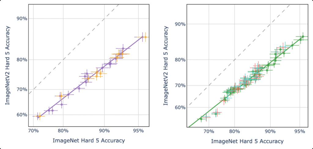
A.2 Probit Scaling

For our scatter plots comparing model accuracies, we follow standard practice and apply probit scaling to the axes (miller2021accuracy) (wortsman2022robust). The probit function is the inverse of the standard normal cumulative distribution function (CDF), ${𝑦}^{\prime }={\mathrm{\Phi }}^{-1}\left(𝑦\right)$ where $𝑦\in \left[0,1\right]$ is the original accuracy and ${𝑦}^{\prime }\in \left[-\infty ,\infty \right]$ is the transformed value.

This transformation is crucial for analyzing accuracy scores, which are bounded between 0 and 1. On a linear scale, the variance of accuracy scores is compressed near the boundaries (e.g., the difference between 98% and 99% appears small). Probit scaling maps the [0, 1] interval to the entire real line, effectively "stretching" the scale at the extremes. This allows for a more meaningful visualization of performance differences between high-performing models and makes linear relationships in performance more apparent across the full range of accuracies.

A.3 Dataset Statistics

To determine a sufficient sample size for stable evaluation, we analyzed model performance on randomly sampled subsets of our benchmark of varying sizes. The results, presented in Table 1, show the accuracy of two representative models, SmolVLM and SmolVLM2, as a function of the number of questions in the ImageNet validation set.

Num	500	1000	2000	5000	8000	10000	20000	30000
SmolVLM	85.2%	85.8%	86.45%	86.72%	87.19%	86.65%	86.92%	86.91%
SmolVLM2	93.6%	94.6%	94.75%	93.7%	93.86%	94.11%	94.05%	94.17%

The data indicates that accuracy scores converge as the sample size increases. Beyond 2,000 samples, the reported accuracy for both models varies by less than 0.5 percentage points. Therefore, our primary test set size is well above the threshold required to produce stable and conclusive results.

A.4 Change Prompt

• Prompt 1: A photo of a {class}
• Prompt 2: {class}
• Prompt 3: What type of object is in this photo?
• Prompt 4: Select the most appropriate label for the object shown in the image.
• Prompt 5: Identify the object in this image.