Reconstruction vs. Generation
1. Generative modelling in latent space
The usual process for training a generative model in latent space consists of two stages:
- Train an autoencoder on the input signals. This is a neural network consisting of two subnetworks, an encoder and a decoder. The former maps an input signal to its corresponding latent representation (encoding). The latter maps the latent representation back to the input domain (decoding).
- Train a generative model on the latent representations. This involves taking the encoder from the first stage, and using it to extract latents for the training data. The generative model is then trained directly on these latents. Nowadays, this is usually either an autoregressive model or a diffusion model.
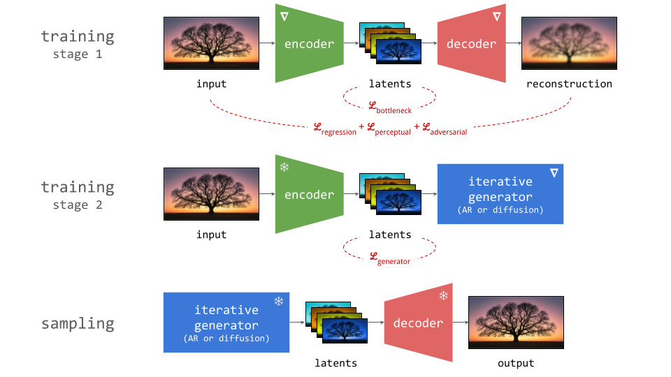
Several different loss functions are involved in the two training stages, which are indicated in red on the diagram:
- To ensure the encoder and decoder are able to convert input representations to latents and back with high fidelity, several loss functions constrain the reconstruction (decoder output) with respect to the input. These usualy include a simple regression loss, a perceptual loss and an adversarial loss.
- To constrain the capacity of the latents, an additional loss function is often applied directly to them during training, although this is not always the case. We will refer to this as the bottleneck loss, because the latent representation forms a bottleneck in the autoencoder network.
- In the second stage, the generative model is trained using its own loss function, separate from those used during the first stage. This is often the negative log-likelihood loss (for autoregressive models), or a diffusion loss.
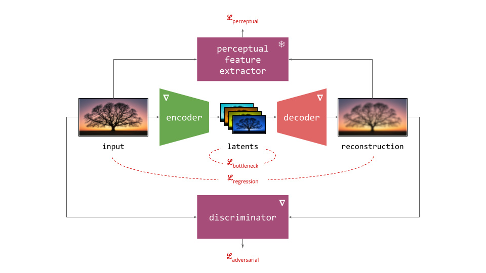
Taking a closer look at the reconstruction-based losses, we have:
- the regression loss, which is sometimes the mean absolute error (MAE) measured in the input space (e.g. on pixels), but more often the mean squared error (MSE).
- the perceptual loss, which can take many forms, but more often than not, it makes use of another frozen pre-trained neural network to extract perceptual features. The loss encourages these features to match between the reconstruction and the input, which results in better preservation of high-frequency content that is largely ignored by the regression loss. LPIPS1 is a popular choice for images.
- the adversarial loss, which uses a discriminator network which is co-trained with the autoencoder, as in generative adversarial networks (GANs). The discriminator is trained to tell apart real input signals from reconstructions, and the autoencoder is trained to fool the discriminator into making mistakes. The goal is to improve the realism of the output, even if it means deviating further from the input signal. It is quite common for the adversarial loss to be disabled for some time at the start of training, to avoid instability.
Below is a more elaborate diagram of the first training stage, explicitly showing the other networks which typically play a role in this process.
1.1. How we got here
The two dominant generative modelling paradigms of today, autoregression and diffusion, were both initially applied to "raw" digital representations of perceptual signals, by which I mean pixels and waveforms.
However, it became clear very quickly that this strategy makes scaling up quite challenging. The most important reason for this can be summarised as follows: perceptual signals mostly consist of imperceptible noise. Or, to put it a different way: out of the total information content of a given signal, only a small fraction actually affects our perception of it. Therefore, it pays to ensure that our generative model can use its capacity efficiently, and focus on modelling just that fraction. That way, we can use smaller, faster and cheaper generative models without compromising on perceptual quality.
1.1.1. Latent regression
Autoregressive models of images took a huge leap forward with the seminal VQ-VAE paper. It suggested a practical strategy for learning discrete representations with neural networks, by inserting a vector quantisation bottleneck layer into an autoencoder. To learn such discrete latents for images, a convolutional encoder with several downsampling stages produced a spatial grid of vectors with a 4× lower resolution than the input (along both height and width, so 16× fewer spatial positions), and these vectors were then quantised by the bottleneck layer.
Now, we could generate images with PixelCNN-style models one latent vector at a time, rather than having to do it pixel by pixel. This significantly reduced the number of autoregressive sampling steps required, but perhaps more importantly, measuring the likelihood loss in the latent space rather than pixel space helped avoid wasting capacity on imperceptible noise.
The discretisation was critical to its success, because autoregressive models were known to work much better with discrete inputs at the time. But perhaps even more importantly, the spatial structure of the latents allowed existing pixel-based models to be adapted very easily. Before this, VAEs (variational autoencoders) would typically compress an entire image into a single latent vector, resulting in a representation without any kind of topological structure. The grid structure of modern latent representations, which mirrors that of the "raw" input representation, is exploited in the network architecture of generative models to increase efficiency (through e.g. convolutions, recurrence or attention layers).
1.1.2. Latent diffusion
An important difference between autoregressive and diffusion models is the loss function used to train them. In the autoregressive case, things are relatively simple: you just maximise the likelihood (although other things have been tried as well). For diffusion, things are a little more interesting: the loss is an expectation over all noise levels, and the relative weighting of these noise levels significantly affects what the model learns. This justifies an interpretation of the typical diffusion loss as a kind of perceptual loss function, which puts more emphasis on signal content that is more perceptually salient.
At first glance, this makes the two-stage approach seem redundant, as it operates in a similar way, i.e. filtering out perceptually irrelevant signal content, to avoid wasting model capacity on it. If we can rely on the diffusion loss to focus only on what matters perceptually, why do we need a separate representation learning stage to filter out the stuff that doesn't? These two mechanisms turn out to be quite complementary in practice however, for two reasons:
- The way perception works at small and large scales, especially in the visual domain, seems to be fundamentally different – to the extent that modelling texture and fine-grained detail merits separate treatment, and an adversarial approach can be more suitable for this.
- Training large, powerful diffusion models is inherently computationally intensive, and operating in a more compact latent space allows us to avoid having to work with bulky input representations. This helps to reduce memory requirements and speeds up training and sampling.
1.2. Why two stages?
As discussed before, it is important to ensure that generative models of perceptual signals can use their capacity efficiently, as this makes them much more cost-effective. This is essentially what the two-stage approach accomplishes: by extracting a more compact representation that focuses on the perceptually relevant fraction of signal content, and modelling that instead of the original representation, we are able to make relatively modestly sized generative models punch above their weight.
The fact that most bits of information in perceptual signals don't actually matter perceptually is hardly a new observation: it is also the key idea underlying lossy compression, which enables us to store and transmit these signals at a fraction of the cost. Compression algorithms like JPEG and MP3 exploit the redundancies present in signals, as well as the fact that our audiovisual senses are more sensitive to low frequencies than to high frequencies, to represent perceptual signals with far fewer bits. (There are other perceptual effects that play a role, such as auditory masking for example, but non-uniform frequency sensitivity is the most important one.)
So why don't we use these lossy compression techniques as a basis for our generative models then? This is not a bad idea, and several works have used these algorithms, or parts of them, for this purpose. But a very natural reflex for people working on generative models is to try to solve the problem with more machine learning, to see if we can do better than these "handcrafted" algorithms.
It's not just hubris on the part of ML researchers, though: there is actually a very good reason to use learned latents, instead of using these pre-existing compressed representations. Unlike in the compression setting, where smaller is better, and size is all that matters, the goal of generative modelling also imposes other constraints: some representations are easier to model than others. It is crucial that some structure remains in the representation, which we can then exploit by endowing the generative model with the appropriate inductive biases. This requirement creates a trade-off between reconstruction quality and modelability of the latents.
An important reason behind the efficacy of latent representations is how they lean in to the fact that our perception works differently at different scales. In the audio domain, this is readily apparent: very rapid changes in amplitude result in the perception of pitch, whereas changes on coarser time scales (e.g. drum beats) can be individually discerned. Less well-known is that the same phenomenon also plays an important role in visual perception: rapid local fluctuations in colour and intensity are perceived as textures. 1
1.3. Trading off reconstruction quality and modelability
The difference between lossy compression and latent representation learning is worth exploring in more detail. One can use machine learning for both, although most lossy compression algorithms in widespread use today do not. These algorithms are typically rooted in rate-distortion theory, which formalises and quantifies the relationship between the degree to which we are able to compress a signal (rate), and how much we allow the decompressed signal to deviate from the original (distortion).
For latent representation learning, we can extend this trade-off by introducing the concept of modelability or learnability, which characterises how challenging it is for generative models to capture the distribution of this representation. This results in a three-way rate-distortion-modelability trade-off, which is closely related to the rate-distortion-usefulness trade-off discussed by Tschannen et al. in the context of representation learning.
It's not immediately obvious why this is even a trade-off at all – why is modelability at odds with distortion? To understand this, consider how lossy compression algorithms operate: they take advantage of known signal structure to reduce redundancy. In the process, this structure is often removed from the compressed representation, because the decompression algorithm is able to reconstitute it. But structure in input signals is also exploited extensively in modern generative models, in the form of architectural inductive biases for example, which take advantage of signal properties like translation equivariance or specific characteristics of the frequency spectrum.
If we have an amazing algorithm that efficiently removes almost all redundancies from our input signals, we are making it very difficult for generative models to capture the unstructured variability that remains in the compressed signals. That is completely fine if compression is all we are after, but not if we want to do generative modelling. So we have to strike a balance: a good latent representation learning algorithm will detect and remove some redundancy, but keep some signal structure as well, so there is something left for the generative model to work with.
A good example of what not to do in this setting is entropy coding, which is actually a lossless compression method, but is also used as the final stage in many lossy schemes (e.g. Huffman coding in JPEG/PNG, or arithmetic coding in H.265). Entropy coding algorithms reduce redundancy by assigning shorter representations to frequently occurring patterns. This doesn't remove any information at all, but it destroys structure. As a result, small changes in input signals could lead to much larger changes in the corresponding compressed signals, potentially making entropy-coded sequences considerably more difficult to model.
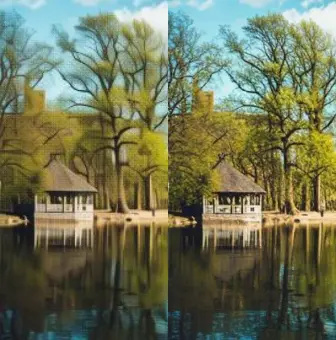
In contrast, latent representations tend to preserve a lot of signal structure. The figure below shows a few visualisations of Stable Diffusion latents for images (taken from the EQ-VAE paper). It is pretty easy to identify the animals just from visually inspecting the latents. They basically look like noisy, low-resolution images with distorted colours. This is why I like to think of image latents as merely "advanced pixels", capturing a little bit of extra information that regular pixels wouldn't, but mostly still behaving like pixels nonetheless.
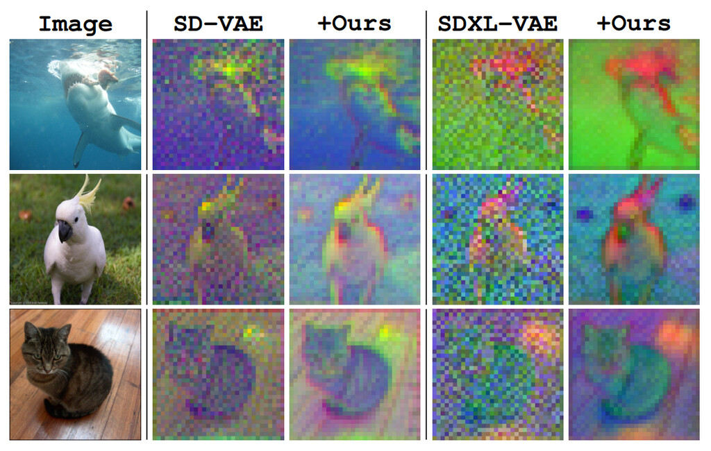
It is safe to say that these latents are quite low-level. Whereas traditional VAEs would compress an entire image into a single feature vector, often resulting in a high-level representation that enables semantic manipulation, modern latent representations used for generative modelling of images are actually much closer to the pixel level. They are much higher-capacity, inheriting the grid structure of the input (though at a lower resolution). Each latent vector in the grid may abstract away some low-level image features such as textures, but it does not capture the semantics of the image content. This is also why most autoencoders do not make use of any additional conditioning signals such as text captions, as those mainly constrain high-level structure (though exceptions exist)
1.4. Controlling capacity
Two key design parameters control the capacity of a grid-structured latent space: the downsampling factor and the number of channels of the representation. If the latent representation is discrete, the codebook size is also important, as it imposes a hard limit on the number of bits information that the latents can contain.
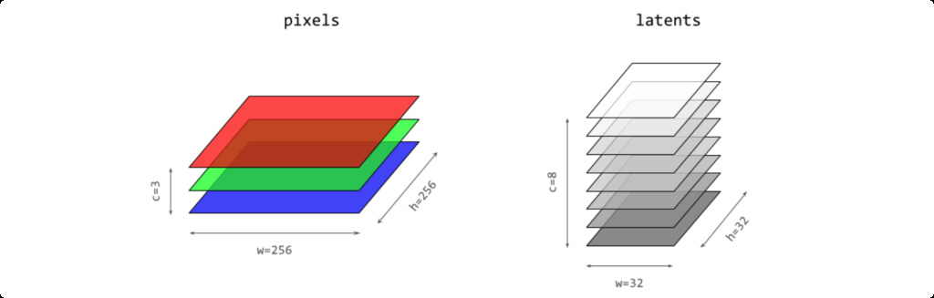
As an example, an encoder might take a 256×256 pixel image as input, and produce a 32×32 grid of continuous latent vectors with 8 channels. This could be achieved using a stack of strided convolutions, or perhaps using a vision Transformer (ViT) with patch size 8. The downsampling factor reduces the dimensionality along both width and height, so there are 64 times fewer latent vectors than pixels – but each latent vector has 8 components, while each pixel has only 3 (RGB). In aggregate, the latent representation is a tensor with times fewer components (i.e. floating point numbers) than the tensor representing the original image. I like to refer to this number as the tensor size reduction factor (TSR), to avoid confusion with spatial or temporal downsampling factors.
From a purely mathematical perspective, this is surprising: if the latents are real-valued, the size of the grid and the number of channels shouldn't matter, because the information capacity of a single number is already infinite (neatly demonstrated by Tupper's self-referential formula). But of course, there are several practical limitations that restrict the amount of information a single component of the latent representation is able to carry:
- we use floating point representations of real numbers, which have finite precision;
- in many formulations, the encoder adds some amount of noise, which further limits effective precision;
- neural networks aren't very good at learning highly nonlinear functions of their input. 2
To recap, choosing the right TSR is key: a larger latent representation will yield better reconstruction quality (higher rate, lower distortion), but may negatively affect modelability. With a larger representation, there are simply more bits of information to model, therefore requiring more capacity in the generative model. In practice, this trade-off is usually tuned empirically. This can be an expensive affair, because there aren't really any reliable proxy metrics for modelability that are cheap to compute. Therefore, it requires repeatedly training large enough generative models to get meaningful results.
1.5. Curating and shaping the latent space
So far, we have talked about the capacity of latent representations, i.e. how many bits of information should go in them. It is just as important to control precisely which bits from the original input signals should be preserved in the latents, and how this information is presented. I will refer to the former as curating the latent space, and to the latter as shaping the latent space – the distinction is subtle, but important. Many regularisation strategies have been devised to shape, curate and control the capacity of latents. I will focus on the continuous case, but many of the same considerations apply to discrete latents as well.
1.5.1. VQGAN and KL-regularised latents
Rombach et al. suggested two regularisation strategies for continuous latent spaces:
- Follow the original VQGAN recipe, reinterpreting the quantisation step as part of the decoder, rather than the encoder, to get a continuous representation (VQ-reg);
- Remove the quantisation step from the VQGAN recipe altogether, and replace it with a KL penalty, as in regular VAEs (KL-reg).
The idea of making only minimal changes to VQGAN to produce continuous latents (for use with diffusion models) is clever: the setup worked well for autoregressive models, and the quantisation during training serves as a safeguard to ensure that the latents don't end up encoding too much information. However, as we discussed previously, this probably isn't really necessary in most cases, because encoder expressivity is usually the limiting factor.
KL regularisation, on the other hand, is a core part of the traditional VAE setup: it is one of the two terms constituting the evidence lower bound (ELBO), which bounds the likelihood from below and enables VAE training to tractably (but indirectly) maximise the likelihood of the data. It encourages the latents to follow the imposed prior distribution (usually Gaussian). Crucially however, the ELBO is only truly a lower bound on the likelihood if there is no scaling hyperparameter in front of this term. Yet almost invariably, the KL term used to regularise continuous latent spaces is scaled down significantly (usually by several orders of magnitude), all but severing the connection with the variational inference context in which it originally arose.
The reason is simple: an unscaled KL term has too strong an effect, imposing a stringent limit on latent capacity and thus severely degrading reconstruction quality. The pragmatic response to that is naturally to scale down its relative contribution to the training loss. (Aside: in settings where one cares less about reconstruction quality, and more about semantic interpretability and disentanglement of the learnt representation, increasing the scale of the KL term can also be fruitful, as in beta-VAE.)
We are veering firmly into opinion territory here, but I feel there is currently quite a bit of magical thinking around the effect of the KL term. It is often suggested that this term encourages the latents to follow a Gaussian distribution, but with the scale factors that are typically used, this effect is way too weak to be meaningful. Even for "proper" VAEs, the aggregate posterior is rarely actually Gaussian.
All of this renders the "V" in "VAE" basically meaningless, in my opinion – its relevance is largely historical. We may as well drop it and talk about KL-regularised autoencoders instead, which more accurately reflects modern practice. The most important effect of the KL term in this setting is to supress outliers and constrain the scale of the latents to some extent. In other words: while the KL term is often presented as constraining capacity, the way it is used in practice mainly constrains the shape of the latents (but even that effect is relatively modest).
1.5.2. Tweaking reconstruction losses
The usual trio of reconstruction losses (regression, perceptual and adversarial) clearly plays an important role in maximising the quality of decoded signals, but it is also worth studying how these losses impact the latents, specifically in terms of curation (i.e. which information they learn to encode). A good latent space in the visual domain makes abstraction of texture to some degree. How do these losses help achieve that?
A useful thought experiment is to consider what happens when we drop the perceptual and adversarial losses, retaining only the regression loss, as in traditional VAEs. This will tend to result in blurry reconstructions. Regression losses do not favour any particular kind of signal content by design, so in the case of images, they will focus on low-frequency content, simply because there is more of it. In natural images, the power of different spatial frequencies tends to be proportional to their inverse square – the higher the frequency, the less power. Since high frequencies constitute only a tiny fraction of the total signal power, the regression loss more strongly rewards accurate prediction of low frequencies than high ones. The relative perceptual importance of these high frequencies is much larger than the fraction of total signal power they represent, and blurry looking reconstructions are the well-known result.
Since texture is primarily composed of precisely these high frequencies which the regression loss largely ignores, we end up with a latent space that doesn't make abstraction of texture, but rather erases textural information altogether. From a perceptual standpoint, that is a particularly undesirable form of latent space curation. This demonstrates the importance of the other two reconstruction loss terms, which ensure that the latents can encode some textural information.
If the regression loss has these undesirable properties, which require other loss terms to mitigate, perhaps we could drop it altogether? It turns out that's not a great idea either, because the perceptual and adversarial losses are much harder to optimise and tend to have pathological local minima (they are usually based on pre-trained neural networks, after all). The regression loss acts as a sort of regulariser, continually providing guardrails against ending up in the bad parts of parameter space as training progresses.
1.6. Representation learning vs. reconstruction
The design choices we have discussed so far usually impact not just reconstruction quality, but also the kind of latent space that is learnt. The reconstruction losses in particular do double duty: they ensure high-quality decoder output, and play an important role in curating the latent space as well. This raises the question whether it is actually desirable to kill two birds with one stone, as we have been doing. I would argue that the answer is no.
Learning a good compact representation for generative modelling on the one hand, and learning to decode that representation back to the input space on the other hand, are two separate tasks. Modern autoencoders are expected to learn to do both at once. The fact that this works reasonably well in practice is certainly a welcome convenience: training an autoencoder is already stage one of a two-stage training process, so ideally we wouldn't want to complicate it any further (although having multiple autoencoder training stages is not unheard of). But this setup also needlessly conflates the two tasks, and some choices that are optimal for one task might not be for the other.
Although the idea of using autoregressive decoders in pixel space, as we did for that paper, has not aged well at all (to put it mildly), I believe using auxiliary decoders to separate the representation learning and reconstruction tasks is still a very relevant idea today. An auxiliary decoder that optimises a different loss, or that has a different architecture (or both), could provide a better learning signal for representation learning and result in better generative modelling performance.
1.6.1. Regularising for modelability
Shaping, curating and constraining the capacity of latents can all affect their modelability:
- Capacity constraints determine how much information is in the latents. The higher the capacity, the more powerful the generative model will have to be to adequately capture all of the information they contain.
- Shaping can be important to enable efficient modelling. The same information can be represented in many different ways, and some are easier to model than others. Scaling and standardisation are important to get right (especially for diffusion models), but higher-order statistics and correlation structure also matter.
- Curation influences modelability, because some kinds of information are much easier to model than others. If the latents encode information about unpredictable noise in the input signal, that will make them less predictable as well.
As discussed earlier, the KL penalty probably doesn't do quite as much to Gaussianise or otherwise smoothen the latent space as many seem to believe. So what can we do instead to make the latents easier to model?
- Use generative priors: co-train a (lightweight) latent generative model with the autoencoder, and make the latents easy to model by backpropagating the generative loss into the encoder, as in LARP or CRT. This requires careful tuning of loss weights, because the generative loss and the reconstruction losses are at odds with each other: latents are easiest to model when they encode no information at all!
- Supervise with pre-trained representations: encourage the latents to be predictive of existing high-quality representations (e.g. DINOv2 features), as in VA-VAE, MAETok or GigaTok.
- Encourage equivariance: make it so that certain transformations of the input (e.g. rescaling, rotations) produce corresponding latent representations that are transformed similarly, as in AuraEquiVAE, EQ-VAE and AF-VAE. Equivariance regularisation makes the latent spectrum more similar to that of the pixel space inputs, which improves modelability.
1.6.2. Diffusion all the way down
A specific class of autoencoders for learning latent representations deserves a closer look: those with diffusion decoders. While a more typical decoder architecture features a feedforward network that directly outputs pixel values in one forward pass, and is trained adversarially, an alternative that's gaining popularity is to use diffusion for the task of latent decoding (as well as for modelling the distribution of the latents). This impacts reconstruction quality, but it also affects what kind of representation is learnt.
SWYCC, -VAE and DiTo are some recent works that explore this approach. They motivate this in a few different ways:
- latents learnt with diffusion decoders provide a more principled, theoretically grounded way of doing hierarchical generative modelling;
- they can be trained with just the MSE loss, which simplifies things and improves robustness (adversarial losses are pretty finicky to tune, after all);
- applying the principle of iterative refinement to decoding improves output quality.
I can't really argue with any of these points, but I do want to point out one significant weakness of diffusion decoders: their computational cost, and the effect this has on decoder latency. I believe one of the key reasons that most commercially deployed diffusion models today are latent models, is that compact latent representations help us avoid iterative refinement in input space, which is slow and costly. Performing the iterative sampling procedure in latent space, and then going back to input space with a single forward pass at the end, is significantly faster.
With that in mind, reintroducing input-space iterative refinement for the decoding task looks to me like it largely defeats the point of the two-stage approach. If we are going to be paying that cost, we might as well opt for something like simple diffusion to scale up single-stage generative models instead.
Not so fast, you might say – can't we use one of the many diffusion distillation methods to bring down the number of steps required? In a setting such as this one, with a very rich conditioning signal (i.e. the latent representation), these methods have indeed proven effective even down to the single-step sampling regime: the stronger the conditioning, the fewer steps are needed for high quality distillation results.
DALL-E 3's consistency decoder is a great practical example of this: they reused the Stable Diffusion latent space and trained a new diffusion-based decoder, which was then distilled down to just two sampling steps using consistency distillation. While it is still more costly than the original adversarial decoder in terms of latency, the visual fidelity of the outputs is significantly improved.
Removing the need for adversarial training would certainly simplify things, so diffusion autoencoders are an interesting (and recently, quite popular) field of study in that regard. Still, it seems challenging to compete with adversarial decoders when it comes to latency, so I don't think we are quite ready to abandon them. I very much look forward to an updated recipe that doesn't require adversarial training, yet matches the current crop of adversarial decoders in terms of both visual quality and latency!
1.7. The tyranny of the grid
Digital representations of perceptual modalities are usually grid-structured, because they arise as uniformly sampled (and quantised) versions of the underlying physical signals. Images give rise to 2D grids of pixels, videos to 3D grids, and audio signals to 1D grids (i.e. sequences). The uniform sampling implies that there is a fixed quantum (i.e. distance or amount of time) between adjacent grid positions.
Perceptual signals also tend to be approximately stationary in time and space in a statistical sense. Combined with uniform sampling, this results in a rich topological structure, which we gratefully take advantage of when designing neural network architectures to process them: we use extensive weight sharing to benefit from invariance and equivariance properties, implemented through convolutions, recurrence and attention mechanisms.
Without a doubt, our ability to exploit this structure is one of the key reasons why we have been able to build machine learning models that are as powerful as they are. A corollary of this is that preserving this structure when designing latent spaces is a great idea. Our most powerful neural network designs architecturally depend on it, because they were originally built to process these digital signals directly. They will be better at processing latent representations instead, if those representations have the same kind of structure.
It also offers significant benefits for the autoencoders which learn to produce the latents: because of the stationarity, and because they only need to learn about local signal structure, they can be trained on smaller crops or segments of input signals. If we impose the right architectural constraints (limiting the receptive field of each position in the encoder and the decoder), they will generalise out of the box to larger grids than they were trained on. This has the potential to greatly reduce the training cost for the first stage.
It's not all sunshine and rainbows though: we have discussed how perceptual signals are highly redundant, and unfortunately, this redundancy is unevenly distributed. Some parts of the signal might contain lots of detail that is perceptually salient, where others are almost devoid of information. In the image of a dog in a field that we used previously, consider a 100×100 pixel patch centered on the dog's head, and then compare that to a 100×100 pixel patch in the top right corner of the image, which contains only the blue sky.
If we construct a latent representation which inherits the 2D grid structure of the input, and use it to encode this image, we will necessarily use the exact same amount of capacity to encode both of these patches. If we make the representation rich enough to capture all the relevant perceptual detail for the dog's head, we will waste a lot of capacity to encode a similar-sized patch of sky. In other words, preserving the grid structure comes at a significant cost to the efficiency of the latent representation.
This is what I call the tyranny of the grid: our ability to process grid-structured data with neural networks is highly developed, and deviating from this structure adds complexity and makes the modelling task considerably harder and less hardware-friendly, so we generally don't do this. But in terms of encoding efficiency, this is actually quite wasteful, because of the non-uniform distribution of perceptually salient information in audiovisual signals.
The Transformer architecture is actually relatively well-positioned to bolster a rebellion against this tyranny: while we often think of it as a sequence model, it is actually designed to process set-valued data, and any additional topological structure that relates elements of a set to each other is expressed through positional encoding. This makes deviating from a regular grid structure more practical than it is for convolutional or recurrent architectures.
Relaxing the topology of the latent space in the context of two-stage generative modelling appears to be gaining some traction lately:
- TiTok and FlowMo learn sequence-structured latents from images, reducing the grid dimensionality from 2D to 1D. The development of large language models has given us extremely powerful sequence models, so this is a reasonable kind of structure to aim for.
- One-D-Piece, FlexTok and Semanticist do the same, but use a nested dropout mechanism to induce a coarse-to-fine structure in the latent sequence. This in turn enables the sequence length to be adapted to the complexity of each individual input image, and to the level of detail required in the reconstruction. A few other mechanisms for adaptive 1D tokenisation have been proposed, e.g. ElasticTok and ALIT. CAT also explores this kind of adaptivity, but still maintains a 2D grid structure and only adapts its resolution.
- TokenSet goes a step further and uses an autoencoder that produces "bags of tokens", abandoning the grid completely.
Aside from CAT, all of these have in common that they learn latent spaces that are considerably more semantically high-level than the ones we have mostly been talking about so far. In terms of abstraction level, they probably sit somewhere in the middle between "advanced pixels" and the vector-valued latents of old-school VAEs. In fact, FlexTok and Semanticist's 1D sequence encoders expect low-level latents from an existing 2D grid-structured encoder as input, literally building an additional abstraction level on top of a pre-existing low-level latent space. TiTok and One-D-Piece also make use of an existing 2D grid-structured latent space as part of a multi-stage training approach. A related idea is to reuse the language domain as a high-level latent representation for images.
In the discrete setting, some work has investigated whether commonly occurring patterns of tokens in a grid can be combined into larger sub-units, using ideas from language tokenisation: DiscreTalk is an early example in the speech domain, using SentencePiece on top of VQ tokens. Zhang et al.'s BPE Image Tokenizer is a more recent incarnation of this idea, using an enhanced byte-pair encoding algorithm on VQGAN tokens.
1.8. Closing thoughts
To wrap up, here are some key takeaways:
- Latents for generative modelling are usually quite unlike VAE latents from way back when: it makes more sense to think of them as advanced pixels than as high-level semantic representations.
- Having two stages enables us to have different loss functions for each, and significantly improves computational efficiency by avoiding iterative sampling in the input space.
- Latents add complexity, but the computational efficiency benefits are large enough for us to tolerate this complexity – at least for now.
- Three main aspects to consider when designing latent spaces are capacity (how many bits of information are encoded in the latents), curation (which bits from the input signals are retained) and shape (how this information is presented).
- Preserving structure (i.e. topology, statistics) in the latent space is important to make it easy to model, even if this is sometimes worse from an efficiency perspective.
- The V in VAE is vestigial: the autoencoders used in two-stage latent generative models are really KL-regularised AEs, and usually barely regularised at that.
- The combination of a regression loss, a perceptual loss and an adversarial loss is surprisingly entrenched. Almost all modern implementations of autoencoders for latent representation learning are variations on this theme.
- Representation learning and reconstruction are two separate tasks, and while it is convenient to do both at once, this might not be optimal.
2. Autoencoders for Diffusion: A Deep Dive
We found that compressing to 1D with a transformer, i.e. just 16 flat vectors, results in good reconstructions that cannot be diffused.
How small can you make this latent? How many channels should it have? What makes one autoencoder good for diffusion models and another bad?
2.1. GANs And The Modern Autoencoder
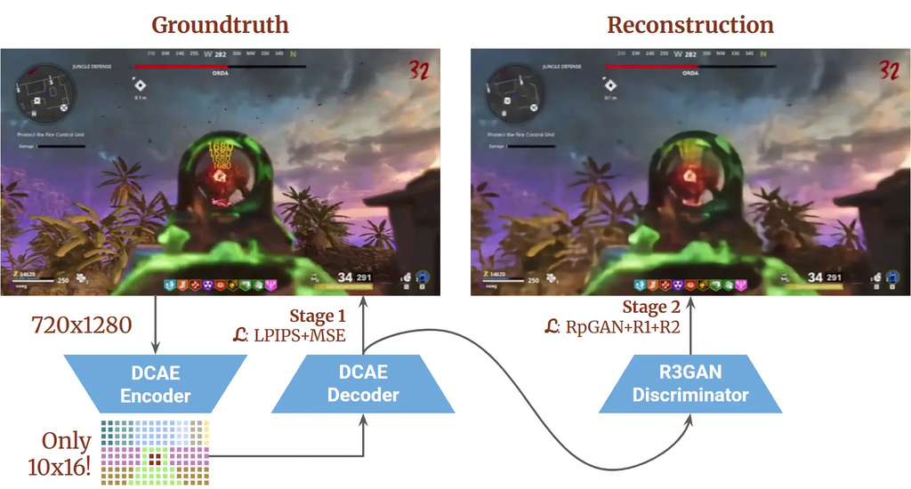
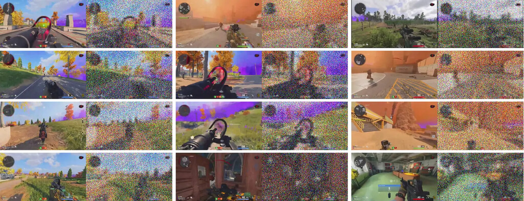
Don't we use diffusion now? Why are GANs relevant? Check out these samples from our 720x1280 10x16 autoencoder:
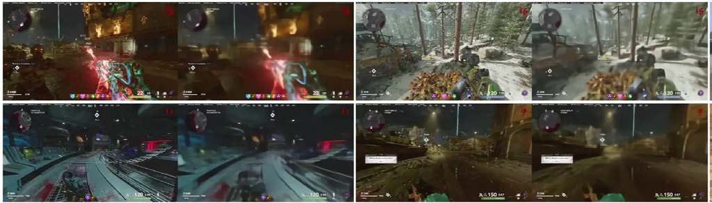
Observe how the reconstructions have a very obvious "blurring" going on. This effect becomes more and more pronounced when you push the latents smaller and smaller. MSE tends to focus too much on the precise positions of things in images, rather than their content, so autoencoders naturally struggle with high frequency 'fine' details. Perceptual losses (we use Conv Next LPIPS) help a little bit but as you can see the blurriness remains. To this end, all modern autoencoders (starting with VQGAN) include an adversarial training phase. The idea is that the GAN loss encourages the autoencoder to generate things it can't reconstruct from its latent. Consider the example of encoding an image of a tree. All trees have leaves and bark, which generally have the same texture/structure. Encoding fine grained details about the bark or leaves wastes valuable bandwidth in the latent space. The DCAE paper shows a very good example of this:
Given the GAN loss is basically telling the model to generate specific details rather than encode them, and we want to be frugal with latent bandwidth, we freeze the encoder during adversarial training in all our GAN training runs. To stay up-to-date on literature we follow a scheme similar to R3GAN, but we will give more details on this shortly.
2.2. Precision Errors In Your VAE? More Likely Than You Think
More constrained activations are naturally desirable if you want to do lower precision for training/inference speed while preserving stability and not being NaN'd into the moon.
Now one point worth bringing up is that it seems to be common knowledge that BF16 is unstable for adversarial training. In the majority of VAE papers, there seems to be no mention of precision. To circumvent instability, many fall back to FP32, reducing training throughput significantly. To us, this isn't a good enough solution. We need more speed!
Following the recipe in R3GAN, we use Fix-Up initialization in the residual blocks within our autoencoder. This means scaling the weights of the convolutions by a factor correlated to the overall number of residual blocks, and the output convolution weights are initialized to zero. Effectively this makes the model start as a sort of "identity", with the residual stream passing through every layer untouched. Of course, when you're downsampling/upsampling, you can't really leave the residual stream untouched. Pixel shuffle and light unbiased 1x1 convolutions can sort of do this, so we take the space to channel and channel to space operations from DCAE and integrate that into our custom architecture.
2.3. Diffusability and Smoothness
Creating a good autoencoder to plug into diffusion models isn't just about reconstruction quality - the latent space needs to be "diffusable," meaning it should be easy for diffusion models to learn and generate from. The properties of your latent space directly impact how well downstream generative models can work with your representations; if your latents are too noisy, have poor spectral characteristics, or contain artifacts from the encoding process, diffusion models will struggle to learn meaningful patterns and generate coherent samples. This is why we focus heavily on ensuring our latents maintain the right properties to make them amenable to diffusion-based generation!
One key aspect of our approach involved implementing spectral equivariance through careful downsampling strategies, following insights from the diffusability of autoencoders paper. This technique helps preserve the spectral characteristics that make latents easier for diffusion models to work with.
Interestingly, we found that contrary to some literature suggesting that increasing channel counts makes autoencoders less diffusable, a channel count of 128 works quite well in our experiments. The key insight from our PCA analysis is that latents should maintain spectral characteristics similar to the original images - they should preserve the distribution of different frequencies that make them "image-like".
Intuitively, we find that as you compress images to smaller latent sizes, the generative task starts to dominate more since the latent space becomes increasingly constrained. This means the model needs to hallucinate more details during reconstruction. Part of our approach involves being careful not to let GAN-specific details leak into the latent space, as this could make the representations less image-like and harder for diffusion models to work with.
It's also worth noting that KL divergence penalties are less commonly used in modern approaches. Instead, many researchers now simply add noise to the inputs during decoder training. We decided against using either approach, figuring that L2 regularization during decoder fine-tuning and post-training should accomplish similar goals without the added complexity.
2.4. Post-Mortem: Proxy Models
Another promising approach was Proxy Models, introduced by the TiToK VQ-VAE image tokenizer paper. The idea is to first train a VQ-VAE to compress a 512x512 image down to 16x16 tokens. Then, train a separate transformer-based VAE that further compresses those 16x16 representations down to just 16 flat tokens (and decoding back to the 16x16 input representation), for a staggering 128x compression!
Unfortunately, this approach didn't work well with diffusion models.
We also experimented with adding a sparsity loss term to the TiToK proxy models. Interestingly, the model learned to effectively ignore about 50% of the 128 latent channels - these values were essentially zeroed out due to the sparsity penalty. We could then manually zero out these unused channels during decoding with no loss in reconstruction quality. However, when we tried training a model with only 64 channels from the start (rather than learning to ignore half of 128 channels), it failed completely. This suggests that having the extra capacity during training is crucial, even if the final learned representation is sparser.
3. Generation vs. Reconstruction: Striking A Balance
We need an autoencoder that can decode 4x4 latents into 360x640 (and eventually 720p) images at 60fps. Naturally, much of the information in the images cannot make its way down into the latents. We are ok with losing information in the latent so long as we can get it back later. With MSE+LPIPS only, this does not happen, and the high frequency bands are cut off, resulting in blurry reconstructions.
Getting high frequency details through the latent is essentially impossible at high compression ratios. On top of this, we need our latent to be as much like a spatial downsample as possible (See our previous blog post for why). These constraints are tight… so how do we do it?
3.1. People Still Use GANs?
For those who are not in the know on diffusion models, GANs might seem dead. Now everyone uses diffusion and autoregression, right? In reality, GANs are still a crucial building block for the modern autoencoder. We explain the motivation behind this in our autoencoder blog post. However, there are some quirks that come with using a GAN signal in your autoencoder. When you introduce the adversarial term, your autoencoder breaks apart into two separate tasks:
-
Downsample the original image into a latent that is informative enough to reconstruct as much of the original image as possible.
-
Use the original image to make a "code" that can be used by a generator to generate an image that fools the discriminator.
3.2. The Rec-Gen Tradeoff
Thus comes the reconstruction-generation tradeoff. For clarity, in the literature this is often used to specify the tradeoff between the autoencoder and the downstream generative model (i.e. diffusion model or autoregressive model). We use it to refer to the autoencoder balancing between being a generator and a reconstructor. In a VAE-GAN, the latent now serves two purposes as we stated earlier. On one hand, it is a downsampled version of the original image, on the other hand it is a code to be used to instruct the decoder on what it should generate. Adversarial weight can directly tune this trade-off, but interestingly enough we have found that the compression factor also indirectly effects it. This makes sense: smaller latents lead to worse reconstructions, which are easier for the discriminator to detect, requiring a stronger generator to actually trick the discriminator. Refer to the following diagram:
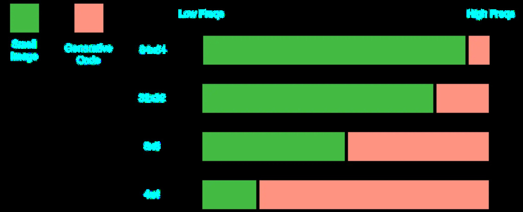
Firstly, as the latent size goes down, the bands of frequency that can be recovered from the latent shrinks, and as a consequence, those frequencies need to instead be generated in order to fool the discriminator. As more and more of the content must be generated, the amount of bandwidth the latent uses for reconstruction (i.e. the "image-like" part) shrinks, while the amount of bandwidth used for generation (i.e. a "code" saying what to generate) goes up. For a VQ-GAN, this is totally fine because the VQ codes are… well… codes. As such this kind of semantic compression actually improves the downstream autoregressive model. However, we've consistently found for diffusion that image-like latents are the best, and deviation from this always introduces problems. In this context, we want to avoid any generative information sneaking into the latent.
3.3. How Do We Get Around This?
Our simple solution is to just decouple generative and reconstructive training. We train the encoder-decoder end-to-end with only reconstructive losses, then freeze+compile the encoder to focus on post-training with the decoder. This has several benefits:
- Without a discriminator, we have a much faster training speed on stage 1
- The latents are fully baked after stage 1, so we can train a WM before even having to worry about stage 2, as it's now just decoder post-training
- Distilling the encoder or the decoder is simple and decoupled from actual autoencoder training
- We can run a variety of experiments for better generative decoders while using the same encoder and latent "api"
- Decoder post-training is much faster when skipping the encoder training
3.4. ResNets are Laggy
On Monday we setup a latency evaluation script in our AVWM training repository. When testing a 1B model with fullgraph compilation on a 5090, we were hitting 350 FPS (assuming KV caching and 1 step generation). However, the image decoder was throttling this bigtime as it was capping out around 50 FPS. This is of course unacceptable for our 60fps target. By dropping all normalization layers (replaced with weightnorms) and the middle block of the autoencoder, we posted performance by a factor of about 1.5x without losing any quality, but it still wasn't ideal. It seemed that convolutions at high resolutions add signifigant overhead.
If it was this bad at 360p, 720p was going to be unattainable. As such, we wanted to explore alternate architectures. So then: what if our decoder was a diffusion transformer?
3.5. Diffusionception
Why diffuse once when you can diffuse twice? After diffusing a latent, we use it as a conditioning signal to diffuse a full RGB image. There is some literature on this, but we felt it seemed too good to be true. Nevertheless, we pressed onwards. At first we introduced a few too many variables. We assumed that
- Since the latent is another "modality" compared to the RGB images, it should be processed separately: we used the MMDiT architecture
- Since mode collapse is entirely fine and every latent should map to a single image anyways, shortcut objective is fine
- Diffusion needs CFG right? We used latent = random noise as a null embedding (which in hindsight doens't really make sense)
- We can just diffuse in RGB space… right?
Our learned landscape-to-square worked for ResNets, so maybe we can just put it at the start and end of our DiT?
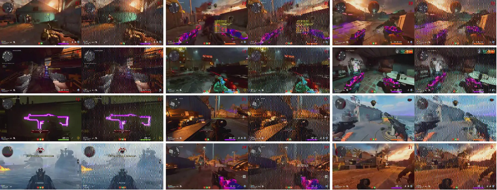
The resulting samples were quite bad, even though it seemed like the model was learning… something:
Upon further discussions with members of our discord community, we removed CFG and trimmed away the MMDiT architecture. This halfed computation during the shortcut step and halfed the model size, without really influencing performance in any regard. Even so, the images remained weird and noisy as you can see above. As a further simplifiying step, we took a page from our failed proxy decoder experiment and attempted to decode not an RGB image, but a Flux Latent. We imagined going from a 4x4 latent to a 64x64 latent was easier than going to a 360x640 RGB image. Initial samples look better but… weird:
We had cut out everything else, we realized it was time to part ways with our beloved aspect ratio convolutions. We instead just did weird patch sizes (p = (5,2) resulting in 360 total tokens). Since we no longer had the square image we couldn't do the pixel shuffle used in Flux to push spatial dims into channel dims (i.e. 64x64 c16 to 32x32 c64). Alas, we simply accepted this and moved on. Finally, we were starting to get samples better than the original autoencoder reconstructions!
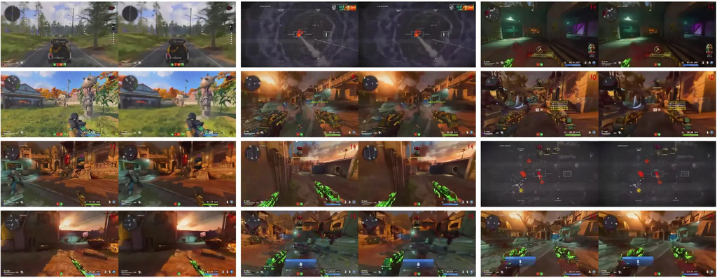
Diffusion models are slow to train, but even at 90k steps, this model is looking quite solid! We are going to wait until 200k to get a better sense of things.
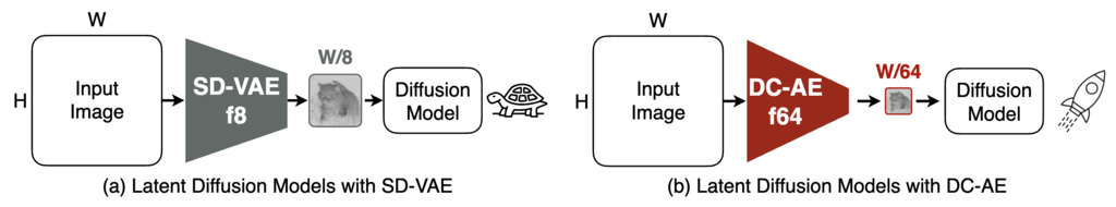
4. DC-AE
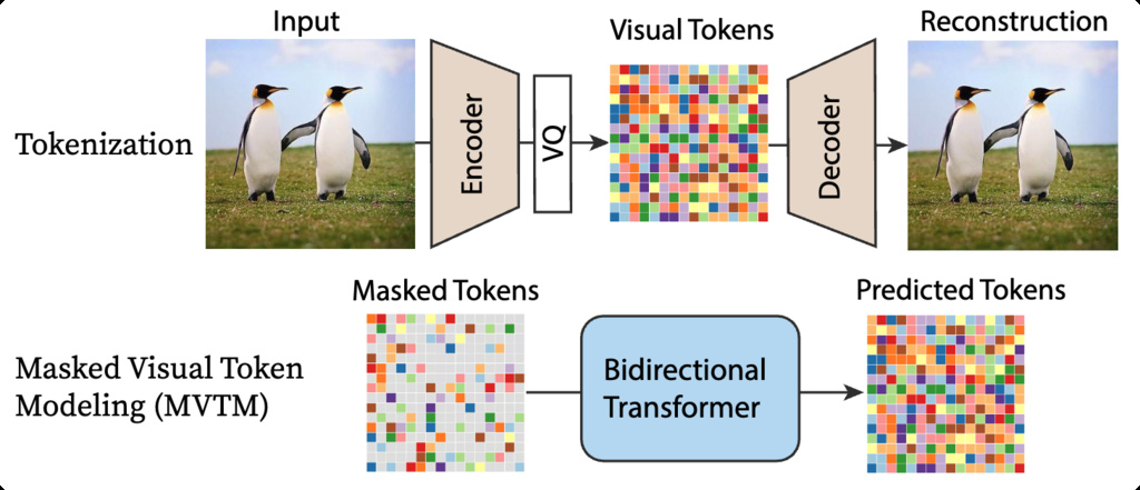
5. Masked Generative Image Transformer (MaskGIT)
MaskGIT adopts a two-stage approach similar to VQGAN:
-
Stage 1: Image Tokenization
- Uses VQGAN's encoder-decoder architecture with vector quantization
- Compresses images into discrete visual tokens (e.g., 256×256 → 16×16 tokens)
- Maintains a codebook of learnable visual vocabulary
-
Stage 2: Masked Visual Token Modeling (MVTM)
- The core innovation involves training a bidirectional transformer to predict masked tokens:
where denote the latent tokens obtained by inputting the image to the VQ-encoder, is the set of masked positions, and is the sequence with masked tokens replaced by [MASK].
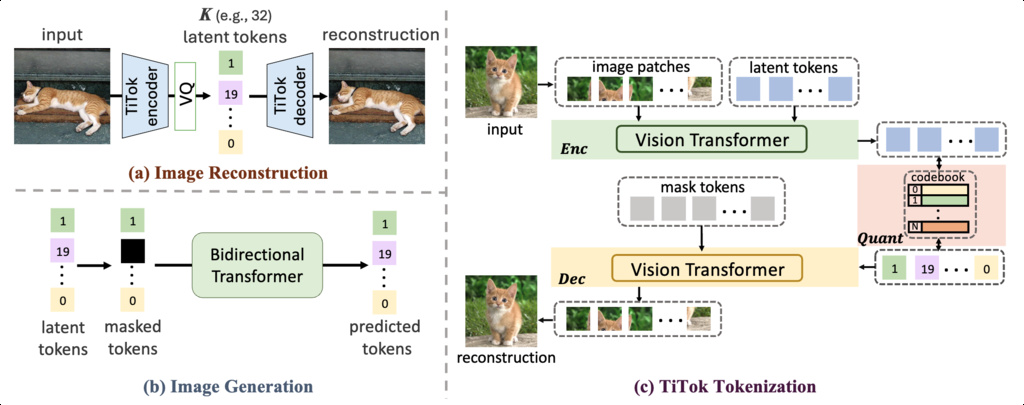
6. Transformer-based 1-Dimensional Tokenizer (TiTok)
Existing image tokenizers, primarily using 2D latent grids (e.g., VQGAN), generate a large number of tokens (256-1024), which limits their ability to fully exploit region redundancy. The large token count from 2D tokenizers leads to high computational demands for training and inference of downstream generative models, hindering scalability and accessibility. It was unclear if compact 1D sequence representations, successful in image understanding, could also capture sufficient detail for high-fidelity image reconstruction and generation.
This paper
- Introduces TiTok, a Transformer-based 1-dimensional tokenizer that represents images with a fixed, small number of latent tokens (e.g., 32), breaking the fixed 2D grid constraint.
- Employs a ViT encoder to distill image information into compact 1D latent tokens, which are then vector-quantized and fed into a ViT decoder for reconstruction using mask tokens.
- Proposes a robust two-stage training paradigm: initial "warm-up" by reconstructing proxy codes from a pre-trained VQGAN, followed by an optional "decoder fine-tuning" directly on pixel space using standard VQGAN losses.
The results show that:
- Increasing the number of latent tokens representing an image consistently improves the reconstruction performance, yet the benefit becomes marginal after 128 tokens. Intriguingly, 32 tokens are sufficient for a reasonable image reconstruction.
- Scaling up the tokenizer model size significantly improves performance of both reconstruction and generation, especially when number of tokens is limited (e.g., 32 or 64), showcasing a promising pathway towards a compact image representation at latent space.
- 1D tokenization breaks the grid constraints in prior 2D image tokenizers, which not only enables each latent token to reconstruct regions beyond a fixed image grid and leads to a more flexible tokenizer design, but also learns more high-level and semantic-rich image information, especially at a compact latent space.
- 1D tokenization exhibits superior performance in generative training, with not only a significant speed-up for both training and inference but also a competitive FID score compared to a typical 2D tokenizer, while using much fewer tokens.
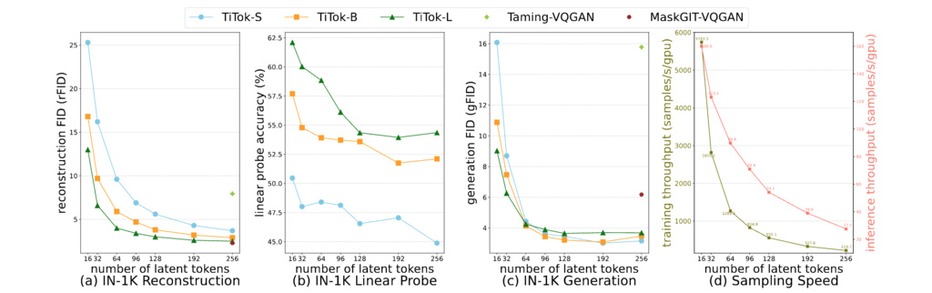
Figure 15:
- Scaling Up Tokenizer Enables More Compact Latent Size. 2. Semantics Emerges with Compact Latent Space. 3. Compact Latent Representation Improves Generative Training.
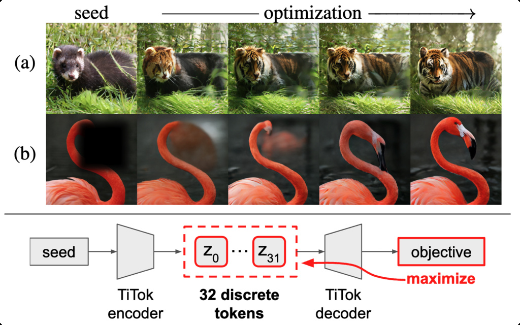
7. Highly Compressed Tokenizer Can Generate Without Training
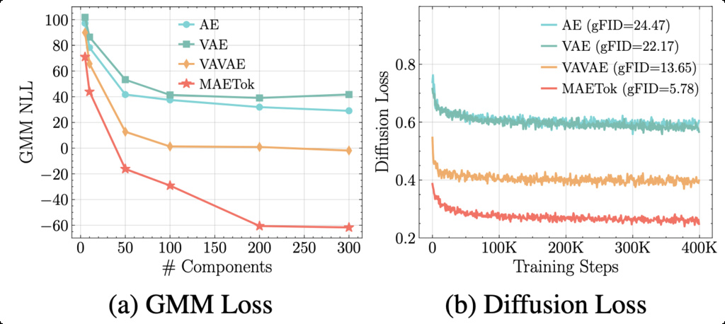
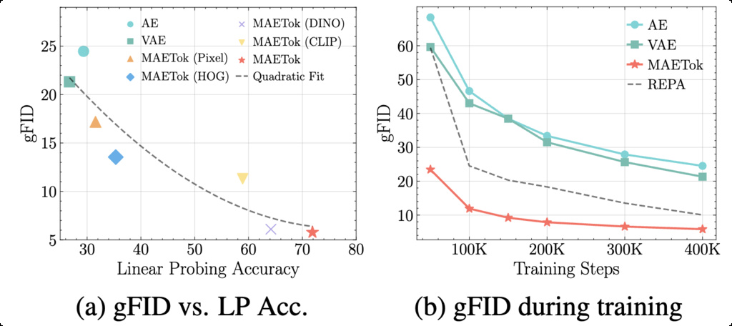
8. MAETok
Variational Autoencoders (VAEs), commonly used as tokenizers in latent diffusion models, often compromise pixel reconstruction fidelity to ensure a smooth latent space. Plain Autoencoders (AEs) achieve higher reconstruction fidelity but traditionally produce less organized latent spaces, considered suboptimal for downstream generative tasks. The specific characteristics of an 'optimal' latent space that enhance diffusion model training efficiency and generation quality remained largely unexplored.
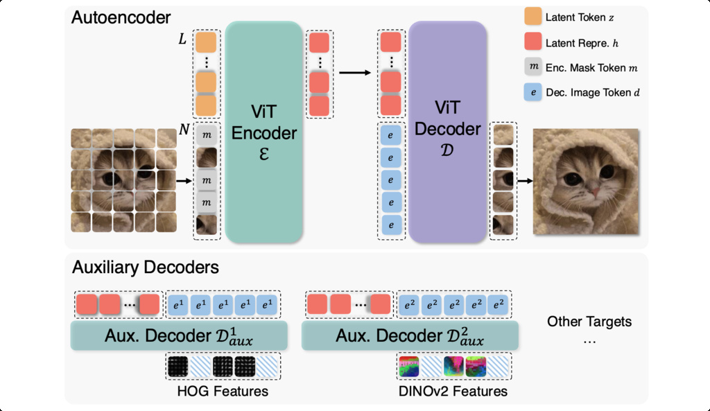
MAETok employs a Vision Transformer (ViT) architecture for both encoder and decoder:
-
Encoder: Takes image patches and learnable latent tokens as input, outputting only the latent representations
-
Decoder: Reconstructs images from latent tokens and learnable image tokens
-
Learnable Tokens: 128 latent tokens provide compressed representation
-
Position Embeddings: 2D Rotary Position Embeddings (RoPE) for image tokens, 1D Absolute Position Embeddings (APE) for latent tokens
-
High Mask Ratio: 40-60% of image patches are randomly masked during encoding
-
Auxiliary Decoders: Multiple shallow decoders predict semantic features (HOG, DINOv2, CLIP) for masked tokens
-
Multi-Target Learning: Forces the encoder to learn robust, semantically rich representations
8.1. Two-Stage Training Process:
-
Stage 1: Masked Autoencoder Training
- Train with high mask ratios and auxiliary decoders
- Focus on learning discriminative latent representations
- Some reconstruction quality may be sacrificed initially
-
Stage 2: Decoder Fine-tuning
- Freeze the encoder to preserve learned latent structure
- Fine-tune only the pixel decoder with gradually decreasing mask ratios
- Recover reconstruction fidelity without compromising latent quality
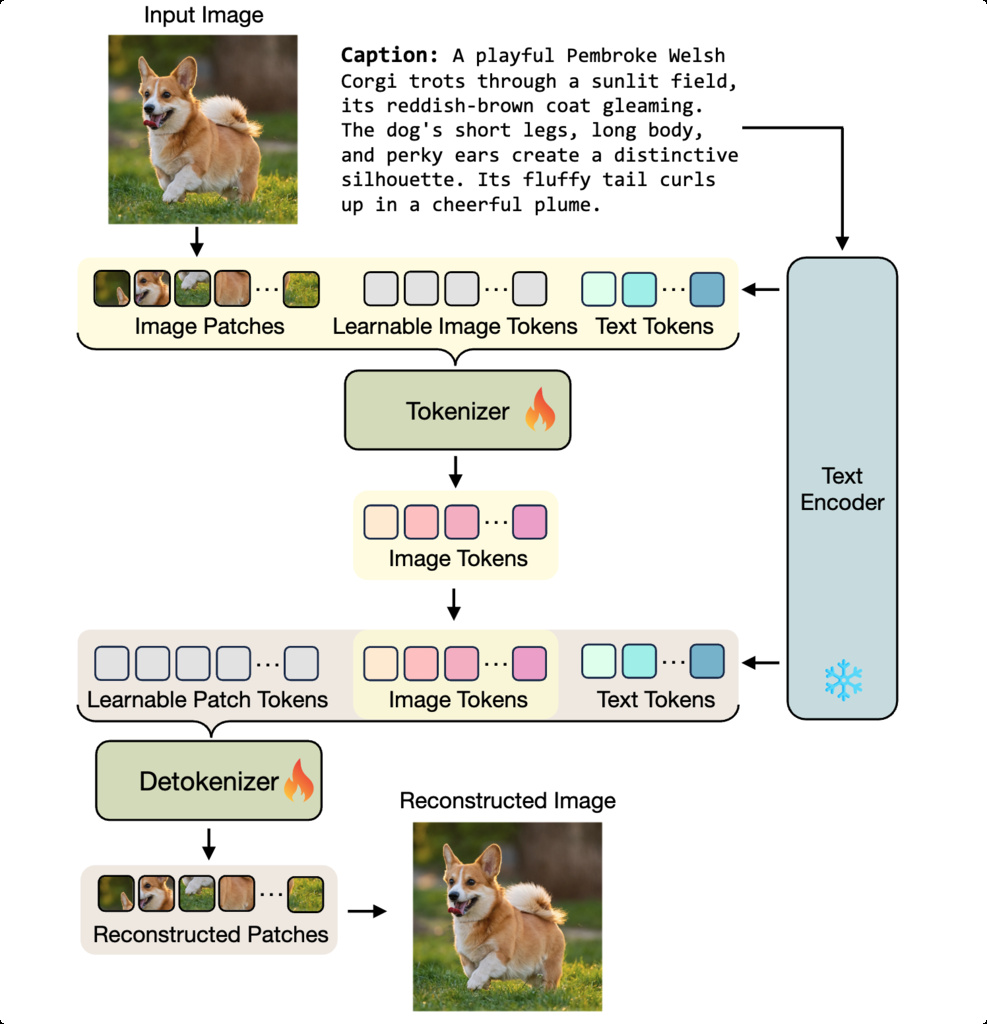
9. TexTok
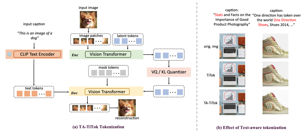
At its core, tokenization involves finding a compact and effective representation of an image. The most concise and meaningful representation of an image often comes from its language description-i.e., captioning. When describing an image, humans naturally start with high-level semantics before elaborating on finer details. Inspired by this insight, we introduce Text-Conditioned Image Tokenization (TexTok), a novel framework that leverages text captions to guide the tokenizer in learning image semantics.
10. UniTok
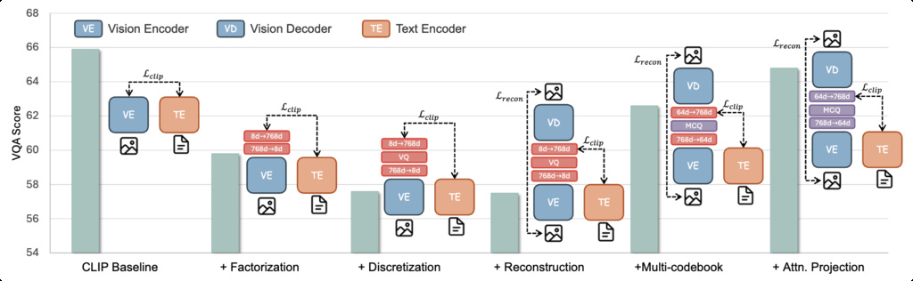
Visual generation models (e.g., VQVAE) and understanding models (e.g., CLIP) traditionally rely on distinct visual tokenizers, hindering true multimodal unification. Previous attempts to unify these objectives by integrating CLIP supervision into VQVAE resulted in perceived "loss conflicts" and suboptimal performance in both generation and understanding. Existing discrete tokenizers suffer from limited representational capacity due to token factorization and coarse discretization, leading to degraded semantic comprehension.
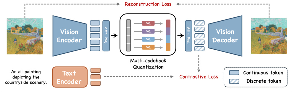
UniTok introduces two key architectural innovations to overcome the discrete token capacity limitation:
- Multi-Codebook Quantization (MCQ): Instead of using a single large codebook, MCQ splits the latent visual vector into multiple smaller chunks, each quantized independently using separate sub-codebooks. For example, with 8 sub-codebooks of 4,096 entries each, the theoretical vocabulary size becomes 32,768, providing exponentially larger representational capacity while maintaining efficient codebook utilization.
- Attention Projection: Replaces simple linear layers for token factorization with adapted multi-head attention modules, better preserving semantic information during dimensionality changes. This addresses the performance degradation observed when compressing high-dimensional features to lower dimensions.
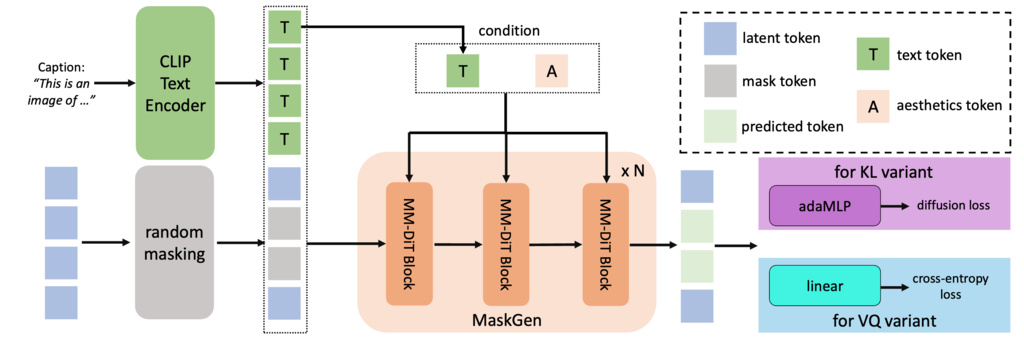
11. Text-Aware Transformer-based 1-Dimensional Tokenizer (TA-TiTok)
-
One way to think of it is texture vs. structure, or sometimes people call this stuff vs. things.
In an image of a dog in a field, the grass texture (stuff) is high-entropy, but we are bad at perceiving differences between individual realisations of this texture, we just perceive it as "grass", in an uncountable sense. We do not need to individually observe each blade of grass to determine that what we're looking at is a field.
If the realisation of this texture is subtly different, we often cannot tell, unless the images are layered directly on top of each other. This is a fun experiment to try with an adversarial autoencoder: when comparing an original image and its reconstruction side by side, they often look identical. But layering them on top of each other and flipping back and forth often reveals just how different the images are, especially in areas with a lot of texture.
For objects (things) on the other hand, like the dog's eyes, for example, differences of a similar magnitude would be immediately obvious.
A good latent representation will make abstraction of texture, but try to preserve structure. That way, the realisation of the grass texture in the reconstruction can be different than the original, without it noticeably affecting the fidelity of the reconstruction. This enables the autoencoder to drop a lot of modes (i.e. other realisations of the same texture) and represent the presence of this texture more compactly in its latent space.
This in turn should make generative modelling in the latent space easier as well, because it can now model the absence/presence of a texture, rather than having to capture all the entropy associated with that texture.
-
The last limitation is actually the more restrictive one, but it is less well understood: isn't the entire point of neural networks to learn nonlinear functions? That is true, but they are naturally biased towards learning relatively simple functions. This is usually a feature, not a bug, because it increases the probability of learning a function that generalises to unseen data. But if we are trying to compress a lot of information into a few numbers, that will likely require a high degree of nonlinearity. There are some ways to assist neural networks with learning more nonlinear functions (such as Fourier features), but in our setting, highly nonlinear mappings will actually negatively affect modelability: they obfuscate signal structure, so this is not a good solution. Representations with more components offer a better trade-off.
References
- Deep Compression Autoencoder for Efficient High-Resolution Diffusion Models
- MaskGIT: Masked Generative Image Transformer
- Reconstruction vs. Generation: Taming Optimization Dilemma in Latent Diffusion Models
- Masked Autoencoders Are Effective Tokenizers for Diffusion Models
- An Image is Worth 32 Tokens for Reconstruction and Generation
- UniTok: A Unified Tokenizer for Visual Generation and Understanding
- Democratizing Text-to-Image Masked Generative Models with Compact Text-Aware One-Dimensional Tokens
- Highly Compressed Tokenizer Can Generate Without Training
- Autoencoders for Diffusion: A Deep Dive
- Generation vs. Reconstruction: Striking A Balance
- Generative modelling in latent space