1. Use latent variable model

$$𝑝\left(𝑥\right)=\int 𝑝\left(𝑥|𝑧\right)𝑝\left(𝑧\right)𝑑𝑧$$$${𝑝}_{𝜃}\left(𝑥|𝑧\right)\to 𝑝\left(𝑥|𝑧\right)$$

$𝑝\left(𝑧\right)$ is the prior distribution, will be a predefined density function.

$$𝑝\left(𝑥\right)=\int 𝑝\left(𝑥|𝑧\right)𝑝\left(𝑧\right)𝑑𝑧$$$$𝑞\left(𝑥|𝑧\right)\to 𝑝\left(𝑥|𝑧\right)$$

$𝑝\left(𝑧\right)$ is the prior distribution, will be a predefined density function.

What we want is to learn ${𝑝}_{𝜃}\left(𝑥|𝑧\right)$ to approximate $𝑝\left(𝑥|𝑧\right)$, which is usually measured by the KL divergence. But its hard to deal with that, so we approximate $𝑝\left(𝑥,𝑧\right)$ instead since $𝑝\left(𝑥,𝑧\right)=𝑝\left(𝑥|𝑧\right)𝑝\left(𝑧\right)$.

$$\begin{array}{cc}\text{KL}\left(𝑝\left(𝑥,𝑧\right)\Vert {𝑝}_{𝜃}\left(𝑥,𝑧\right)\right)& =\iint 𝑝\left(𝑥,𝑧\right)\log \left(\frac{𝑝\left(𝑥,𝑧\right)}{{𝑝}_{𝜃}\left(𝑥,𝑧\right)}\right)𝑑𝑥𝑑𝑧\\ & =\int 𝑝\left(𝑥\right)\left[\int 𝑝\left(𝑧|𝑥\right)\log \frac{𝑝\left(𝑥\right)𝑝\left(𝑧|𝑥\right)}{{𝑝}_{𝜃}\left(𝑥,𝑧\right)}𝑑𝑧\right]𝑑𝑥\\ & ={𝐸}_{𝑥\sim 𝑝\left(𝑥\right)}\left[\int 𝑝\left(𝑧|𝑥\right)\left(\log 𝑝\left(𝑥\right)+\log \frac{𝑝\left(𝑧|𝑥\right)}{{𝑝}_{𝜃}\left(𝑥,𝑧\right)}\right)𝑑𝑧\right]\\ & ={𝐸}_{𝑥\sim 𝑝\left(𝑥\right)}\left[\log 𝑝\left(𝑥\right)\int 𝑝\left(𝑧|𝑥\right)𝑑𝑧\right]+{𝐸}_{𝑥\sim 𝑝\left(𝑥\right)}\left[\int 𝑝\left(𝑧|𝑥\right)\log \frac{𝑝\left(𝑧|𝑥\right)}{{𝑝}_{𝜃}\left(𝑥,𝑧\right)}𝑑𝑧\right]\\ & ={𝐸}_{𝑥\sim 𝑝\left(𝑥\right)}\left[\log 𝑝\left(𝑥\right)\right]-{𝐸}_{𝑥\sim 𝑝\left(𝑥\right)}\left[\int 𝑝\left(𝑧|𝑥\right)\log \frac{{𝑝}_{𝜃}\left(𝑥,𝑧\right)}{𝑝\left(𝑧|𝑥\right)}𝑑𝑧\right]\\ \end{array}$$

The first term is a constant, so we only need to maximize the second term:

$$\begin{array}{cc}ℒ& ={𝐸}_{𝑥\sim 𝑝\left(𝑥\right)}\left[\int 𝑝\left(𝑧|𝑥\right)\log \frac{{𝑝}_{𝜃}\left(𝑥,𝑧\right)}{𝑝\left(𝑧|𝑥\right)}𝑑𝑧\right]\\ & ={𝐸}_{𝑥\sim 𝑝\left(𝑥\right)}\left[\int 𝑝\left(𝑧|𝑥\right)\log \frac{{𝑝}_{𝜃}\left(𝑥|𝑧\right)𝑝\left(𝑧\right)}{𝑝\left(𝑧|𝑥\right)}𝑑𝑧\right]\\ & ={𝐸}_{𝑥\sim 𝑝\left(𝑥\right)}\left[\int 𝑝\left(𝑧|𝑥\right)\log {𝑝}_{𝜃}\left(𝑥|𝑧\right)𝑑𝑧+\int 𝑝\left(𝑧|𝑥\right)\log \frac{𝑝\left(𝑧\right)}{𝑝\left(𝑧|𝑥\right)}𝑑𝑧\right]\\ & ={𝐸}_{𝑥\sim 𝑝\left(𝑥\right)}\left[{𝐸}_{𝑧\sim 𝑝\left(𝑧|𝑥\right)}\left[\log {𝑝}_{𝜃}\left(𝑥|𝑧\right)\right]\right]-\text{KL}\left(𝑝\left(𝑧|𝑥\right)\Vert 𝑝\left(𝑧\right)\right)\\ \end{array}$$

This is Evidence Lower Bound (ELBO). But is maximizing the ELBO similar to doing maximum likelihood estimation (MLE)? Yes, since we can show that

$$\begin{array}{cc}{𝐸}_{𝑥\sim 𝑝\left(𝑥\right)}\left[\text{ELBO}\left(𝑥\right)\right]& ={𝐸}_{𝑥\sim 𝑝\left(𝑥\right)}\left[\int 𝑝\left(𝑧|𝑥\right)\log \frac{{𝑝}_{𝜃}\left(𝑥,𝑧\right)}{𝑝\left(𝑧|𝑥\right)}𝑑𝑧\right]\\ & ={𝐸}_{𝑥\sim 𝑝\left(𝑥\right)}\left[\int 𝑝\left(𝑧|𝑥\right)\log \frac{{𝑝}_{𝜃}\left(𝑥\right){𝑝}_{𝜃}\left(𝑧|𝑥\right)}{𝑝\left(𝑧|𝑥\right)}𝑑𝑧\right]\\ & ={𝐸}_{𝑥\sim 𝑝\left(𝑥\right)}\left[\log {𝑝}_{𝜃}\left(𝑥\right)\right]-\text{KL}\left(𝑝\left(𝑧|𝑥\right)\Vert {𝑝}_{𝜃}\left(𝑧|𝑥\right)\right)]\end{array}$$

1.1. VAE

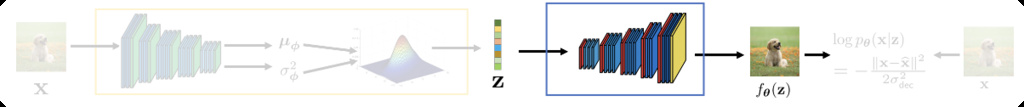
We choose $𝑝\left(𝑧\right)$ to be $𝒩\left(0,1\right)$, and use networks to approximate $𝑝\left(𝑧|𝑥\right)$ and $𝑝\left(𝑥|𝑧\right)$.

$$\begin{array}{c}\left(𝜇,{𝜎}^2\right)={\text{ EncoderNetwork }}_{𝜑}\left(𝑥\right),\\ {𝑞}_{𝜑}\left(𝑧|𝑥\right)=𝒩\left(𝑧|𝜇,\text{ diag}\left({𝜎}^2\right)\right)\end{array}$$

$𝑝\left(𝑥|𝑧\right)$ is one-to-one mapping. We use ${𝑝}_{𝜃}\left(𝑥|𝑧\right)=𝛿\left(𝑥-{𝑓}_{𝜃}\left(𝑧\right)\right)$ to approximate $𝑝\left(𝑥|𝑧\right)$.

$$\begin{array}{c}{𝑓}_{𝜃}\left(𝑧\right)={\text{ DecoderNetwork }}_{𝜃}\left(𝑧\right),\\ {𝑝}_{𝜃}\left(𝑥|𝑧\right)=𝒩\left(𝑥|{𝑓}_{𝜃}\left(𝑧\right),{𝜎}_{\text{ dec }}^2𝐼\right)\end{array}$$

where ${𝜎}_{\text{dec}}$ is a hyperparameter. Thus the first term of the loss function is

$$\begin{array}{cc}{𝐸}_{𝑥\sim 𝑝\left(𝑥\right)}\left[{𝐸}_{𝑧\sim {𝑞}_{𝜑}\left(𝑧|𝑥\right)}\left[-\log {𝑝}_{𝜃}\left(𝑥|𝑧\right)\right]\right]& ={𝐸}_{𝑥\sim 𝑝\left(𝑥\right)}\left[{𝐸}_{𝑧\sim {𝑞}_{𝜑}\left(𝑧|𝑥\right)}\left[-\log \frac{1}{\sqrt{2𝜋}{𝜎}_{\text{ dec}}}\exp \left(-\frac{{\left(𝑥-{𝑓}_{𝜃}\left(𝑧\right)\right)}^2}{2{𝜎}_{\text{ dec}}^2}\right)\right]\right]\\ & =\frac{1}{2{𝜎}_{\text{ dec}}^2}{𝐸}_{𝑥\sim 𝑝\left(𝑥\right)}\left[{𝐸}_{𝑧\sim {𝑞}_{𝜑}\left(𝑧|𝑥\right)}\left[{\left(𝑥-{𝑓}_{𝜃}\left(𝑧\right)\right)}^2\right]\right]-\log \frac{1}{\sqrt{2𝜋}{𝜎}_{\text{ dec}}}\end{array}$$

Since $\text{KL}\left({𝑁}_0\Vert {𝑁}_1\right)=\frac{1}{2}\left(\mathrm{tr}\left({\sum }_1^{-1}{\sum }_0\right)+{\left({𝜇}_1-{𝜇}_0\right)}^{𝑇}{\sum }_1^{-1}\left({𝜇}_1-{𝜇}_0\right)+\log \frac{\left|{\sum }_1\right|}{\left|{\sum }_0\right|}-𝑘\right)$, the second term is

$$\text{KL}\left({𝑞}_{𝜑}\left(𝑧|𝑥\right)\Vert 𝑝\left(𝑧\right)\right)=\frac{1}{2}\left(-\log {𝜎}^2+{𝜇}^2+{𝜎}^2-1\right)$$

We are trying to find $\left(𝜑,𝜃\right)=\arg \underset{𝜑,𝜃}{\max }{𝐸}_{𝑥\sim 𝑝\left(𝑥\right)}\left[\text{ELBO}\left(𝑥\right)\right]$.

1.1.1. Conditioned VAE (CVAE)

We define ${𝐿}_{\text{CVAE }}={𝐸}_{\left(𝑥,𝑦\right)\sim 𝑝\left(𝑥,𝑦\right)}\left[{𝐸}_{𝑧\sim {𝑞}_{𝜑}\left(𝑧|𝑥,𝑦\right)}\left[\log {𝑝}_{𝜃}\left(𝑦|𝑥,𝑧\right)\right]\right]-\text{KL}\left({𝑞}_{𝜑}\left(𝑧|𝑥,𝑦\right)\Vert {𝑝}_{𝜃}\left(𝑧|𝑥\right)\right)$ and also Gaussian stochastic neural network (GSNN) with loss ${𝐿}_{\text{GSNN }}={𝐸}_{\left(𝑥,𝑦\right)\sim 𝑝\left(𝑥,𝑦\right)}\left[{𝐸}_{𝑧\sim {𝑞}_{𝜑}\left(𝑧|𝑥\right)}\left[\log {𝑝}_{𝜃}\left(𝑦|𝑥,𝑧\right)\right]\right]$. The total loss is ${𝐿}_{\text{hybrid }}=𝛼{𝐿}_{\text{ CVAE }}+\left(1-𝛼\right){𝐿}_{\text{ GSNN}}$.

1.1.2. $𝛽$-VAE

$ℒ={𝐸}_{𝑥\sim 𝑝\left(𝑥\right)}\left[{𝐸}_{𝑧\sim {𝑞}_{𝜑}\left(𝑧|𝑥\right)}\left[\log {𝑝}_{𝜃}\left(𝑥|𝑧\right)\right]\right]-𝛽\text{KL}\left({𝑞}_{𝜑}\left(𝑧|𝑥\right)\Vert 𝑝\left(𝑧\right)\right)$, when $𝛽>1$, each dimension of $𝑧\sim {𝑞}_{𝜑}\left(𝑧|𝑥\right)$ are forced to be more independent (disentangled).

1.1.3. VAE with Discrete Latent

1.1.3.1. Gumbel-Softmax

Gumbel Max is a way to sample from a categorical distribution. We assume the probability of each category is ${𝑝}_{𝑖}$, then $\arg \underset{𝑖}{\max }\left(\log {𝑝}_{𝑖}-\log \left(-\log {𝜀}_{𝑖}\right)\right),{𝜀}_{𝑖}\sim 𝑈\left[0,1\right]$ is equivalent to sampling from the categorical distribution, which is a reparametrization trick.

But $\arg \max$ is not differentiable, so we use softmax to approximate it:

$$\text{softmax}\left(\frac{\log {𝑝}_{𝑖}-\log \left(-\log {𝜀}_{𝑖}\right)}{𝜏}\right),{𝜀}_{𝑖}\sim 𝑈\left[0,1\right]$$

Where $𝜏$ is a temperature parameter. The smaller $𝜏$, the more likely the result is to be one-hot.

Using Gumbel-Softmax, we can use $𝑝\left(𝑧\right)=\text{uniform}\left(0,𝑘-1\right)$ instead of $𝑝\left(𝑧\right)=𝒩\left(0,1\right)$.

1.1.3.2. Vector-Quantization VAE (VQ-VAE)

Reduce dimensions and use PixelCNN to generate images.

In reality, we encoder $𝑥$ into a $𝑚\times 𝑚$ grid of $𝑑$-dimensional vectors. But $\arg \min$ is not differentiable, so we use Straight-Through Estimator to define our own gradient and change loss function:

$${\Vert 𝑥-\text{decoder}\left({𝑧}_{𝑞}\right)\Vert }_2^2\to {\Vert 𝑥-\text{decoder}\left(𝑧+\text{ sg}\left[{𝑧}_{𝑞}-𝑧\right]\right)\Vert }_2^2$$

To make ${𝑧}_{𝑞}$ more similar to $𝑧$, we can add ${\Vert 𝑧-{𝑧}_{𝑞}\Vert }_2^2$ to the loss function. Decompose ${\Vert {𝑧}_{𝑞}-𝑧\Vert }_2^2$ into ${\Vert \text{sg}\left[𝑧\right]-{𝑧}_{𝑞}\Vert }_2^2+{\Vert 𝑧-\text{sg}\left[𝑧\right]\Vert }_2^2$. The first term fixes $𝑧$ and makes ${𝑧}_{𝑞}$ closer to $𝑧$ and the second term makes $𝑧$ closer to ${𝑧}_{𝑞}$. Since ${𝑧}_{𝑞}$ is more free to change, so the loss function is:

$${\Vert 𝑥-\text{decoder}\left(𝑧+\text{ sg}\left[{𝑧}_{𝑞}-𝑧\right]\right)\Vert }_2^2+𝛽{\Vert \text{sg}\left[𝑧\right]-{𝑧}_{𝑞}\Vert }_2^2+𝛾{\Vert 𝑧-\text{sg}\left[{𝑧}_{𝑞}\right]\Vert }_2^2$$

where $𝛾<𝛽$. After training, we can use $𝑝\left(𝑧\right)$ to train auto-regressive models like PixelCNN for better sampling.

1.1.3.3. VQ-VAE 2

Bi-level VQ-VAE, bottom level conditions on top level.

1.1.3.4. DALL-E

Discrete VAE using ResNet with 8192 codebook size & 1024 image tokens.

1.1.3.5. DALL-E 2/3

Image generation model over image embeddings.

1.1.3.6. Latent Diffusion Models (LDM)

dVAE + Transformer prior over large-scale text-image paired data