1. KL Divergence and its variants

$\text{KL}\left(𝑃\Vert 𝑄\right)={𝐸}_{𝑥\sim 𝑃}\left[\log \frac{𝑃\left(𝑥\right)}{𝑄\left(𝑥\right)}\right]$

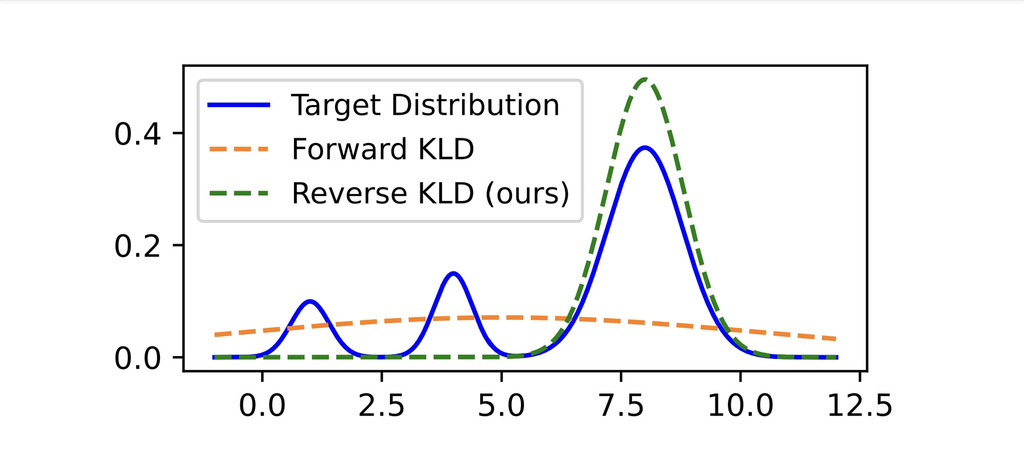
Forward (inclusive) KL: $\text{KL}\left(𝑃\Vert 𝑄\right)$ where $𝑃$ is the true distribution and $𝑄$ is the approximating distribution.

• Mode covering: Since we sample from $𝑃$ and penalize when $𝑄\left(𝑥\right)$ is small, $𝑄$ tends to cover all modes of $𝑃$ (even if it means being over-dispersed). If $𝑃\left(𝑥\right)>0$ but $𝑄\left(𝑥\right)\approx 0$, the penalty is large.
• Typical use: Maximize likelihood, VAE (ensures decoder explains all data)

Reverse (exclusive) KL: $\text{KL}\left(𝑄\Vert 𝑃\right)$

• Mode seeking: Since we sample from $𝑄$ and penalize when $𝑃\left(𝑥\right)$ is small, $𝑄$ tends to concentrate on a single mode of $𝑃$ (under-dispersed but sharper). If $𝑄\left(𝑥\right)>0$ but $𝑃\left(𝑥\right)\approx 0$, the penalty is large.
• Reduces exposure bias ¹
• Typical use: Variational inference, policy optimization in RL

1.1. Jensen-Shannon Divergence

$$\text{JSD}\left(𝑃\Vert 𝑄\right)=\frac{1}{2}\left(\text{KL}\left(𝑃\Vert 𝑀\right)+\text{ KL}\left(𝑄\Vert 𝑀\right)\right),𝑀=\frac{1}{2}\left(𝑃+𝑄\right)$$

JSD measures divergence relative to the mixture distribution $𝑀$, which makes it:

• Symmetric: $\text{JSD}\left(𝑃\Vert 𝑄\right)=\text{JSD}\left(𝑄\Vert 𝑃\right)$ (unlike KL)
• Bounded: $0\le \text{JSD}\left(𝑃\Vert 𝑄\right)\le 1$ (log 2 when distributions have disjoint support)
• Nearly a metric: $\sqrt{\text{JSD}\left(𝑃\Vert 𝑄\right)}$ satisfies triangle inequality
• Balances between mode-covering and mode-seeking behavior of KL variants

1.2. Wasserstein Distance

The distribution of $𝑇\left(𝑥\right)$ is called the push-forward of $𝑃$, denoted by ${𝑇}_{\#}𝑃\left(𝐴\right)=𝑃\left(\left\{𝑥:𝑇\left(𝑥\right)\in 𝐴\right\}\right)=𝑃\left({𝑇}^{-1}\left(𝐴\right)\right)$

The Monge version of the optimal transport distance is $\underset{𝑇}{\inf }\int {\Vert 𝑥-𝑇\left(𝑥\right)\Vert }^{𝑝}𝑑𝑃\left(𝑥\right)$ where the infimum is over all $𝑇$ such that ${𝑇}_{\#}𝑃=𝑄$. Intuitively, this measures how far you have to move the mass of $𝑃$ to turn it into $𝑄$. A minimizer ${𝑇}^{\ast }$, if one exists, is called the optimal transport map.

Let $\mathrm{\Pi }\left(𝑃,𝑄\right)$ denote all joint distributions $𝜋$ for $\left(𝑋,𝑌\right)$ that have marginals $𝑃$ and $𝑄$. In other words, ${𝑇}_{𝑋\#}𝜋=𝑃$ and ${𝑇}_{𝑌\#}𝜋=𝑄$ where ${𝑇}_{𝑋}\left(𝑥,𝑦\right)=𝑥$ and ${𝑇}_{𝑌}\left(𝑥,𝑦\right)=𝑦$. Then the Wasserstein distance is

$${𝑊}_{𝑝}\left(𝑃,𝑄\right)={\left(\underset{𝛾\in \mathrm{\Pi }\left(𝑃,𝑄\right)}{\inf }\int {\Vert 𝑥-𝑦\Vert }^{𝑝}𝑑𝛾\left(𝑥,𝑦\right)\right)}^{\frac{1}{𝑝}}={\left(\underset{𝛾\in \mathrm{\Pi }\left(𝑃,𝑄\right)}{\inf }{𝐸}_{𝑥,𝑦\sim 𝛾}\left[{\Vert 𝑥-𝑦\Vert }^{𝑝}\right]\right)}^{\frac{1}{𝑝}}$$

where $𝑝\ge 1$. When $𝑝=1$, this is also called the Earth Mover's Distance.

It can be shown from Kantorovich Rubinstein Duality that

$${𝑊}_{𝑝}^{𝑝}\left(𝑃,𝑄\right)=\sum _{𝜓,𝜑}\int 𝜓\left(𝑦\right)𝑑𝑄\left(𝑦\right)-\int 𝜑\left(𝑥\right)𝑑𝑃\left(𝑥\right)$$

where $𝜓\left(𝑦\right)-𝜑\left(𝑥\right)\le {\Vert 𝑥-𝑦\Vert }^{𝑝}$. When $𝑝=1$, we have

$${𝑊}_1\left(𝑃,𝑄\right)=\underset{{\Vert 𝑇\Vert }_{𝐿}\le 1}{\sup }{𝐸}_{𝑥\sim 𝑃}\left[𝑇\left(𝑥\right)\right]-{𝐸}_{𝑦\sim 𝑄}\left[𝑇\left(𝑦\right)\right]$$

where ${\Vert 𝑇\Vert }_{𝐿}\le 1$ means $\left|𝑇\left(𝑥\right)-𝑇\left(𝑦\right)\right|\le \Vert 𝑥-𝑦\Vert$.

When to use Wasserstein Distance instead of KL:

• Non-overlapping distributions: KL divergence becomes infinite (or undefined) when distributions have non-overlapping support, while WD remains finite and meaningful. This is critical in high-dimensional spaces where distributions rarely overlap perfectly.
• Meaningful gradients: Even when distributions barely overlap, WD provides useful gradients for optimization. This is why Wasserstein GAN (WGAN)) works better than vanilla GAN - it can still learn when the generator distribution is far from the real data distribution.
• True metric: WD is a proper distance metric (satisfies triangle inequality), making it more suitable for geometric interpretations and certain theoretical analyses.
• Weak topology: WD convergence is weaker than KL convergence, meaning $𝑊\left({𝑃}_{𝑛},𝑃\right)\to 0$ implies convergence in distribution, which is often more natural for generative modeling.

1.3. Fisher Divergence

$$𝐹\left(𝑃\Vert 𝑄\right)=\frac{1}{2}{𝐸}_{𝑥\sim 𝑃}\left[{\Vert {\nabla }_{𝑥}\log 𝑃\left(𝑥\right)-{\nabla }_{𝑥}\log 𝑄\left(𝑥\right)\Vert }_2^2\right]$$

Unlike KL divergence which compares probability values, Fisher divergence compares the score functions (gradients of log probabilities). This makes it particularly useful when:

• Dealing with unnormalized distributions (only need score functions, not normalization constants)
• Training score-based generative models
• The score function is more well-behaved than the density itself

1.4. Applications

• Variational Inference: Reverse KL (mode-seeking behavior prevents over-dispersed approximations)
• GAN: JSD (symmetric, bounded measure between real and generated distributions)
• WGAN: Wasserstein Distance (stable training with meaningful gradients)
• VAE: Forward KL (mode-covering ensures all data modes are explained)
• RL (e.g., PPO, TRPO): Reverse KL (prevents policy from assigning probability to bad actions)
• Score-based models (diffusion): Fisher Divergence (training without normalized densities)