1. Flow map matching (FMM)

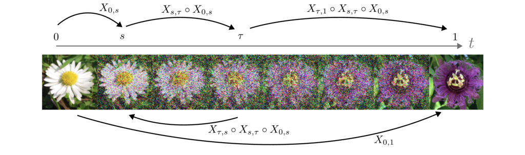
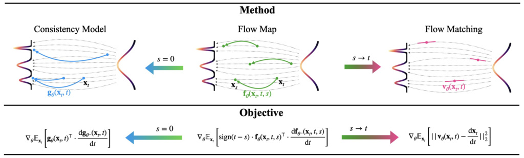
The central object in our method is the flow map, which maps points along trajectories of solutions to an ordinary differential equation (ODE)

1.1. Stochastic interpolants and probability flows

Stochastic interpolant: ${𝐼}_{𝑡}={𝛼}_{𝑡}{𝑥}_0+{𝛽}_{𝑡}{𝑥}_1+{𝛾}_{𝑡}𝑧$, where ${𝛼}_0={𝛽}_1=1,{𝛼}_1={𝛽}_0=0$, and ${𝛾}_0={𝛾}_1=0$.

Probability flow: The probability density of ${𝐼}_{𝑡}$ is the solution to

$${\dot{𝑥}}_{𝑡}={𝑏}_{𝑡}\left({𝑥}_{𝑡}\right),{𝑥}_{𝑡=0}={𝑥}_0\sim {𝜌}_0$$

where ${𝑏}_{𝑡}\left(𝑥\right)=𝐸\left[{\dot{𝐼}}_{𝑡}|{𝐼}_{𝑡}=𝑥\right]$. The drift $𝑏$ can be learned efficiently in practice by solving a square loss regression problem

$$𝑏=\underset{\widehat{𝑏}}{\mathrm{argmin}}{\int }_0^1𝐸\left[{\left|{\widehat{𝑏}}_{𝑡}\left({𝐼}_{𝑡}\right)-{\dot{𝐼}}_{𝑡}\right|}^2\right]𝑑𝑡$$

1.2. Flow map: definition and characterizations

Flow map: The flow map ${𝑋}_{𝑠,𝑡}:{𝑅}^{𝑑}\to {𝑅}^{𝑑}$ is the unique map such that

$${𝑋}_{𝑠,𝑡}\left({𝑥}_{𝑠}\right)={𝑥}_{𝑡}\text{ for all }\left(𝑠,𝑡\right)\in {\left[0,1\right]}^2,$$

where ${\left({𝑥}_{𝑡}\right)}_{𝑡\in \left[0,1\right]}$ is any solution to the ODE.

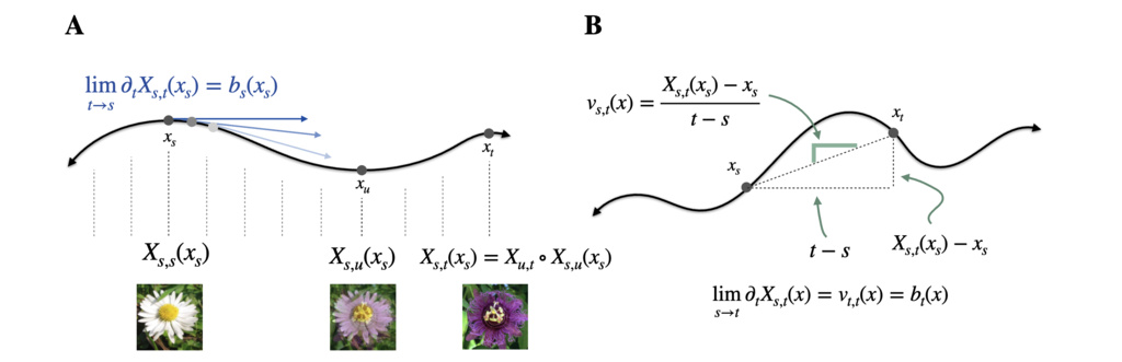
Tangent condition: Let ${𝑋}_{𝑠,𝑡}$ denote the flow map. Then

$$\underset{𝑠\to 𝑡}{\lim }{\partial }_{𝑡}{𝑋}_{𝑠,𝑡}\left(𝑥\right)={𝑏}_{𝑡}\left(𝑥\right)\forall 𝑡\in \left[0,1\right],\forall 𝑥\in {𝑅}^{𝑑}.$$

We define ${𝑣}_{𝑠,𝑡}$ as the exact remainder obtained by truncating a Taylor expansion in $𝑡-𝑠$ of ${𝑋}_{𝑠,𝑡}\left(𝑥\right)$ at first order

$${𝑋}_{𝑠,𝑡}\left(𝑥\right)=𝑥+\left(𝑡-𝑠\right){𝑣}_{𝑠,𝑡}\left(𝑥\right),{𝑣}_{𝑡,𝑡}\left(𝑥\right)={𝑏}_{𝑡}\left(𝑥\right)$$

Geometrically, ${𝑣}_{𝑠,𝑡}$ describes the “slope” of the line drawn between ${𝑥}_{𝑠}$ and ${𝑥}_{𝑡}$ on a single ODE trajectory.

Some of its useful properties: The flow map ${𝑋}_{𝑠,𝑡}\left(𝑥\right)$ is the unique solution to the Lagrangian equation

$${\partial }_{𝑡}{𝑋}_{𝑠,𝑡}\left(𝑥\right)={𝑏}_{𝑡}\left({𝑋}_{𝑠,𝑡}\left(𝑥\right)\right),{𝑋}_{𝑠,𝑠}\left(𝑥\right)=𝑥,$$

for all $\left(𝑠,𝑡,𝑥\right)\in {\left[0,1\right]}^2\times {\mathrm{ℝ}}^{𝑑}$. In addition, it satisfies

$${𝑋}_{𝑡,𝜏}\left({𝑋}_{𝑠,𝑡}\left(𝑥\right)\right)={𝑋}_{𝑠,𝜏}\left(𝑥\right)$$

for all $\left(𝑠,𝑡,𝜏,𝑥\right)\in {\left[0,1\right]}^3\times {\mathrm{ℝ}}^{𝑑}$. In particular, ${𝑋}_{𝑠,𝑡}\left({𝑋}_{𝑠,𝑡}\left(𝑥\right)\right)=𝑥$ for all $\left(𝑠,𝑡,𝑥\right)\in {\left[0,1\right]}^2\times {\mathrm{ℝ}}^{𝑑}$, i.e., the flow map is invertible.

The flow map ${𝑋}_{𝑠,𝑡}$ is the unique solution of the Eulerian equation,

$${\partial }_{𝑡}{𝑋}_{𝑠,𝑡}\left(𝑥\right)+{𝑏}_{𝑠}\left(𝑥\right)·\nabla {𝑋}_{𝑠,𝑡}\left(𝑥\right)=0,{𝑋}_{𝑠,𝑠}\left(𝑥\right)=𝑥,$$

for all $\left(𝑠,𝑡,𝑥\right)\in {\left[0,1\right]}^2\times {\mathrm{ℝ}}^{𝑑}$.

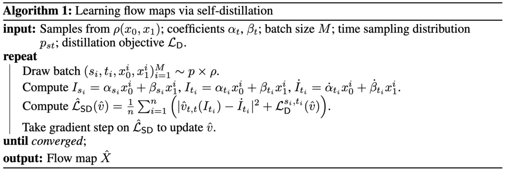
1.3. Flow map training

1.3.1. Distillation of a known velocity field

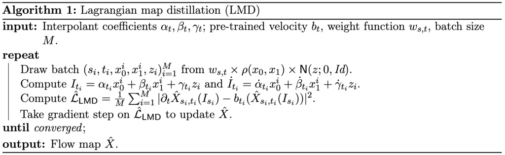
Lagrangian map distillation: Let ${𝑤}_{𝑠,𝑡}\in {𝐿}^1\left({\left[0,1\right]}^2\right)$ be a weight function satisfying ${𝑤}_{𝑠,𝑡}>0$ and let ${𝐼}_{𝑠}$ be the stochastic interpolant. Then the flow map is the global minimizer over $\widehat{𝑋}$ of the loss

$${ℒ}_{\text{LMD}}\left(\widehat{𝑋}\right)={\int }_{{\left[0,1\right]}^2}{𝑤}_{𝑠,𝑡}𝐸\left[{\left|{\partial }_{𝑡}{\widehat{𝑋}}_{𝑠,𝑡}\left({𝐼}_{𝑠}\right)-{𝑏}_{𝑡}\left({\widehat{𝑋}}_{𝑠,𝑡}\left({𝐼}_{𝑠}\right)\right)\right|}^2\right]𝑑𝑠𝑑𝑡,$$

subject to the boundary condition that ${\widehat{𝑋}}_{𝑠,𝑠}\left(𝑥\right)=𝑥$ for all $𝑥\in {𝑅}^{𝑑}$ and $𝑠\in \left[0,1\right]$. $𝐸$ denotes an expectation over the coupling $\left({𝑥}_0,{𝑥}_1\right)\sim {𝜌}_0\left({𝑥}_0,{𝑥}_1\right)$ and $𝑧\sim 𝑁\left(0,{𝐼}_{𝑑}\right)$.

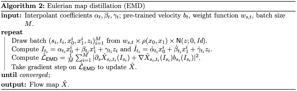
Eulerian map distillation: The flow map is the global minimizer over $\widehat{𝑋}$ of the loss

$${ℒ}_{\text{EMD}}\left(\widehat{𝑋}\right)={\int }_{{\left[0,1\right]}^2}{𝑤}_{𝑠,𝑡}𝐸\left[{\left|{\partial }_{𝑠}{\widehat{𝑋}}_{𝑠,𝑡}\left({𝐼}_{𝑠}\right)+{𝑏}_{𝑠}\left({𝐼}_{𝑠}\right)·\nabla {\widehat{𝑋}}_{𝑠,𝑡}\left({𝐼}_{𝑠}\right)\right|}^2\right]𝑑𝑠𝑑𝑡,$$

1.3.1.1. From Distillation to Direct Training: The stopgrad Necessity

The distillation losses ${ℒ}_{\text{LMD}}$ and ${ℒ}_{\text{EMD}}$ assume that we have access to the true, smooth drift field ${𝑏}_{𝑡}$. A natural question arises: what if ${𝑏}_{𝑡}$ is unknown and we only have access to samples from the stochastic interpolant, including the noisy velocity ${\dot{𝐼}}_{𝑡}$?

A naive approach might be to simply replace the true drift ${𝑏}_{𝑠}$ with its single-sample, noisy estimate ${\dot{𝐼}}_{𝑠}$ in the loss function. For example, the Eulerian loss would become:

$${ℒ}_{\text{Naive}}\left(\widehat{𝑋}\right)={\int }_{{\left[0,1\right]}^2}{𝑤}_{𝑠,𝑡}𝐸\left[{\left|{\partial }_{𝑠}{\widehat{𝑋}}_{𝑠,𝑡}\left({𝐼}_{𝑠}\right)+{\dot{𝐼}}_{𝑠}·\nabla {\widehat{𝑋}}_{𝑠,𝑡}\left({𝐼}_{𝑠}\right)\right|}^2\right]𝑑𝑠𝑑𝑡,$$

However, this naive objective is flawed and will not converge to the correct flow map $𝑋$.

The issue lies in the relationship ${𝑏}_{𝑠}\left(𝑥\right)=𝐸\left[{\dot{𝐼}}_{𝑠}|{𝐼}_{𝑠}=𝑥\right]$. The term ${\dot{𝐼}}_{𝑠}$ is a random variable, while ${𝑏}_{𝑠}\left({𝐼}_{𝑠}\right)$ is its conditional mean. Due to the property $𝐸\left[{𝑌}^2\right]={\left(𝐸\left[𝑌\right]\right)}^2+\text{Var}\left(𝑌\right)$, the naive loss implicitly contains an extra variance term:

$$\begin{array}{cc}& 𝐸\left[{\left|{\partial }_{𝑠}\widehat{𝑋}+{\dot{𝐼}}_{𝑠}·\nabla \widehat{𝑋}\right|}^2\right]\\ & =𝐸\left[{\left|{\partial }_{𝑠}\widehat{𝑋}+{𝑏}_{𝑠}·\nabla \widehat{𝑋}\right|}^2\right]+𝐸\left[\text{Var}\left({\dot{𝐼}}_{𝑠}·\nabla \widehat{𝑋}|{𝐼}_{𝑠}\right)\right]\end{array}$$

This extra variance term acts as a penalty that depends on $\nabla \widehat{𝑋}$. To minimize the total loss, the optimizer is incentivized to find a solution $\widehat{𝑋}$ with an artificially small gradient $\nabla \widehat{𝑋}$, leading to a biased and incorrect result.

To counteract this, a common technique is to use a stop-gradient operator. The operator, stopgrad(z), allows z to pass through during the forward pass but blocks gradients from flowing back through it during optimization. A corrected Eulerian loss would look like:

$${ℒ}_{\text{EE }}=\int {𝑤}_{𝑠,𝑡}𝐸\left[{\left|{\partial }_{𝑠}{\widehat{𝑋}}_{𝑠,𝑡}\left({𝐼}_{𝑠}\right)+\text{stopgrad}\left({\dot{𝐼}}_{𝑠}·\nabla {\widehat{𝑋}}_{𝑠,𝑡}\left({𝐼}_{𝑠}\right)\right)\right|}^2\right]𝑑𝑠𝑑𝑡$$

By blocking the gradient from the noisy term, we can ensure that the expected gradient of the loss is zero at the true solution, making it a valid objective.

This challenge of handling noisy velocities directly is a primary motivation for developing more sophisticated objectives like Flow Map Matching (FMM), which we introduce next. FMM provides an alternative, well-posed loss function for direct training.

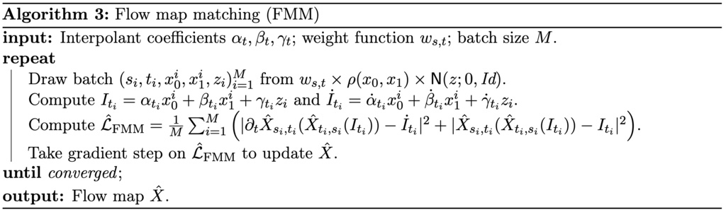
1.3.2. Direct training with flow map matching (FMM)

Flow map matching: The flow map is the global minimizer over $\widehat{𝑋}$ of the loss

$${ℒ}_{\text{FMM}}\left(\widehat{𝑋}\right)={\int }_{{\left[0,1\right]}^2}{𝑤}_{𝑠,𝑡}\left(𝐸\left[{\left|{\partial }_{𝑡}{\widehat{𝑋}}_{𝑠,𝑡}\left({\widehat{𝑋}}_{𝑡,𝑠}\left({𝐼}_{𝑡}\right)\right)-{\dot{𝐼}}_{𝑡}\right|}^2\right]+𝐸\left[{\left|{\widehat{𝑋}}_{𝑠,𝑡}\left({\widehat{𝑋}}_{𝑡,𝑠}\left({𝐼}_{𝑡}\right)\right)-{𝐼}_{𝑡}\right|}^2\right]\right)𝑑𝑠𝑑𝑡,$$

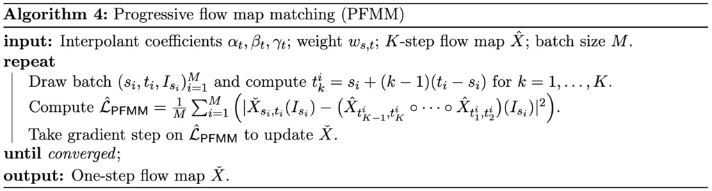
1.3.3. Progressive distillation

Progressive flow map matching: Let $\widehat{𝑋}$ be a two-time flow map. Given $𝐾\in \mathrm{\mathbb{N}}$, let ${𝑡}_{𝑘}=𝑠+\frac{𝑘-1}{𝐾-1}\left(𝑡-𝑠\right)$ for $𝑘=1,\dots ,𝐾$. Then the objective

$${ℒ}_{\text{PFMM}}\left(\widehat{𝑋}\right)={\int }_{{\left[0,1\right]}^2}{𝑤}_{𝑠,𝑡}𝐸\left[{\left|{\widehat{𝑋}}_{𝑠,𝑡}\left({𝐼}_{𝑠}\right)-\left({\widehat{𝑋}}_{{𝑡}_{𝐾-1},{𝑡}_{𝐾}}\circ {\widehat{𝑋}}_{{𝑡}_{𝐾-2},{𝑡}_{𝐾-1}}\circ \dots \circ {\widehat{𝑋}}_{{𝑡}_1,{𝑡}_2}\right)\left({𝐼}_{𝑠}\right)\right|}^2\right]𝑑𝑠𝑑𝑡,$$

produces the same output in one step as the $𝐾$-step iterated map $\widehat{𝑋}$.

1.3.4. Self-distillation

Self-distillation: The flow map ${𝑋}_{𝑠,𝑡}$ is given for all $0\le 𝑠\le 𝑡\le 1$ by ${𝑋}_{𝑠,𝑡}=𝑥+\left(𝑡-𝑠\right){𝑣}_{𝑠,𝑡}\left(𝑥\right)$ where ${𝑣}_{𝑠,𝑡}\left(𝑥\right)$ the unique minimizer over $\widehat{𝑣}$ of

$${ℒ}_{𝑆𝐷}\left(\widehat{𝑣}\right)={ℒ}_{𝑏}\left(\widehat{𝑣}\right)+{ℒ}_{𝐷}\left(\widehat{𝑣}\right),$$

where ${ℒ}_{𝑏}\left(\widehat{𝑣}\right)$ is given by

$${ℒ}_{𝑏}\left(\widehat{𝑣}\right)={\int }_0^1{𝐸}_{{𝑥}_0,{𝑥}_1}\left[{\left|{\widehat{𝑣}}_{𝑡,𝑡}\left({𝐼}_{𝑡}\right)-{\dot{𝐼}}_{𝑡}\right|}^2\right]𝑑𝑡,$$

and where ${ℒ}_{𝐷}\left(\widehat{𝑣}\right)$ is any linear combination of the following three objectives:

(i) The Lagrangian self-distillation (LSD) objective,

$${ℒ}_{𝐷}^{\text{LSD}}\left(\widehat{𝑣}\right)={\int }_0^1{\int }_0^{𝑡}{𝐸}_{{𝑥}_0,{𝑥}_1}\left[{\left|{\partial }_{𝑡}{\widehat{𝑋}}_{𝑠,𝑡}\left({𝐼}_{𝑠}\right)-{\widehat{𝑣}}_{𝑡,𝑡}\left({\widehat{𝑋}}_{𝑠,𝑡}\left({𝐼}_{𝑠}\right)\right)\right|}^2\right]𝑑𝑠𝑑𝑡,$$

(ii) The Eulerian self-distillation (ESD) objective,

$${ℒ}_{𝐷}^{\text{ESD}}\left(\widehat{𝑣}\right)={\int }_0^1{\int }_0^{𝑡}{𝐸}_{{𝑥}_0,{𝑥}_1}\left[{\left|{\partial }_{𝑠}{\widehat{𝑋}}_{𝑠,𝑡}\left({𝐼}_{𝑠}\right)+\nabla {\widehat{𝑋}}_{𝑠,𝑡}\left({𝐼}_{𝑠}\right){\widehat{𝑣}}_{𝑡,𝑡}\left({𝐼}_{𝑠}\right)\right|}^2\right]𝑑𝑠𝑑𝑡;$$

(iii) The progressive self-distillation (PSD) objective,

$${ℒ}_{𝐷}^{\text{PSD}}\left(\widehat{𝑣}\right)={\int }_0^1{\int }_0^{𝑡}{\int }_{𝑠}^{𝑡}{𝐸}_{{𝑥}_0,{𝑥}_1}\left[{\left|{\widehat{𝑋}}_{𝑠,𝑡}\left({𝐼}_{𝑠}\right)-{\widehat{𝑋}}_{𝑢,𝑡}\left({\widehat{𝑋}}_{𝑠,𝑢}\left({𝐼}_{𝑠}\right)\right)\right|}^2\right]𝑑𝑢𝑑𝑠𝑑𝑡.$$

Above, ${\widehat{𝑋}}_{𝑠,𝑡}\left(𝑥\right)=𝑥+\left(𝑡-𝑠\right){\widehat{𝑣}}_{𝑠,𝑡}\left(𝑥\right)$ and ${𝐸}_{{𝑥}_0,{𝑥}_1}$ denotes an expectation over the random draw of $\left({𝑥}_0,{𝑥}_1\right)$.

1.3.5. Align your flow (AYF)

The first training objective aims to ensure that for a fixed $𝑠$, the output of the flow map remains constant as we move $\left({𝑥}_{𝑡},𝑡\right)$ along the PF-ODE.

AYF-Eulerian Map Distillation (AYF-EMD): Let ${𝑓}_{𝜃}\left({𝑥}_{𝑡},𝑡,𝑠\right)$ be the flow map. Consider the loss function defined between two adjacent starting time steps $𝑡$ and ${𝑡}^{\prime }=𝑡+𝜀\left(𝑠-𝑡\right)$ for a small $𝜀>0$,

$${𝐸}_{{𝑥}_{𝑡},𝑡,𝑠}\left[𝑤\left(𝑡,𝑠\right){\Vert {𝑓}_{𝜃}\left({𝑥}_{𝑡},𝑡,𝑠\right)-{𝑓}_{{𝜃}^{-}}\left({𝑥}_{{𝑡}^{\prime }},{𝑡}^{\prime },𝑠\right)\Vert }_2^2\right],$$

where ${𝑥}_{{𝑡}^{\prime }}$ is obtained by applying a 1-step Euler solver to the PF-ODE from $𝑡$ to ${𝑡}^{\prime }$. In the limit as $𝜀\to 0$, the gradient of this loss function with respect to $𝜃$ gives

$${\nabla }_{𝜃}{𝐸}_{{𝑥}_{𝑡},𝑡,𝑠}\left[{𝑤}^{\prime }\left(𝑡,𝑠\right)\text{ sign}\left(𝑡-𝑠\right)\cdot {𝑓}_{𝜃}^{𝑇}\left({𝑥}_{𝑡},𝑡,𝑠\right)\cdot \frac{𝑑{𝑓}_{{𝜃}^{-}}\left({𝑥}_{𝑡},𝑡,𝑠\right)}{𝑑𝑡}\right]$$

where ${𝑤}^{\prime }\left(𝑡,𝑠\right)=𝑤\left(𝑡,𝑠\right)\times \left|𝑡-𝑠\right|$. The AYF-EMD loss naturally generalizes the loss used to train continuous-time consistency models, as it reduces to the same objective when $𝑠=0$.

The second approach ensures consistency at timestep $𝑠$ instead. This method tries to ensure that for a fixed $\left({𝑥}_{𝑡},𝑡\right)$, the trajectory ${𝑓}_{𝜃}\left({𝑥}_{𝑡},𝑡,·\right)$ is aligned with that points' PF-ODE.

AYF-Lagrangian Map Distillation (AYF-LMD): Let ${𝑓}_{𝜃}\left({𝑥}_{𝑡},𝑡,𝑠\right)$ be the flow map. Consider the loss function defined between two adjacent ending timesteps $𝑠$ and ${𝑠}^{\prime }=𝑠+𝜀\left(𝑡-𝑠\right)$ for a small $𝜀>0$,

$${𝐸}_{{𝑥}_{𝑡},𝑡,𝑠}\left[𝑤\left(𝑡,𝑠\right){\Vert {𝑓}_{𝜃}\left({𝑥}_{𝑡},𝑡,𝑠\right)-{\text{ ODE}}_{{𝑠}^{\prime }\to 𝑠}\left({𝑓}_{{𝜃}^{-}}\left({𝑥}_{𝑡},𝑡,{𝑠}^{\prime }\right)\right)\Vert }_2^2\right],$$

where ${\text{ODE}}_{𝑡\to 𝑠}\left(𝑥\right)$ refers to running a 1-step Euler solver on the PF-ODE starting from $𝑥$ at timestep $𝑡$ to timestep $𝑠$. In the limit as $𝜀\to 0$, the gradient of this objective with respect to $𝜃$ converges to:

$${\nabla }_{𝜃}{𝐸}_{{𝑥}_{𝑡},𝑡,𝑠}\left[{𝑤}^{\prime }\left(𝑡,𝑠\right)\text{ sign}\left(𝑠-𝑡\right)\cdot {𝑓}_{𝜃}^{𝑇}\left({𝑥}_{𝑡},𝑡,𝑠\right)\cdot \left(\frac{𝑑{𝑓}_{{𝜃}^{-}}\left({𝑥}_{𝑡},𝑡,𝑠\right)}{𝑑𝑠}-{𝑣}_{𝜑}\left({𝑓}_{{𝜃}^{-}}\left({𝑥}_{𝑡},𝑡,𝑠\right),𝑠\right)\right)\right],$$

where ${𝑤}^{\prime }\left(𝑡,𝑠\right)=𝑤\left(𝑡,𝑠\right)\times \left|𝑡-𝑠\right|$.

References

1. Flow map matching with stochastic interpolants: A mathematical framework for consistency models
2. How to build a consistency model: Learning flow maps via self-distillation
3. Align Your Flow: Scaling Continuous-Time Flow Map Distillation