1. Elucidating the Design Space of Diffusion-Based Generative Models

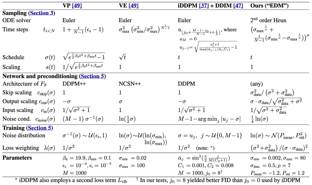
Elucidating the Design Space of Diffusion-Based Generative Models (EDM) provides the first comprehensive theoretical and empirical analysis of the design choices that define these powerful generative systems.

1.1. Unified Mathematical Framework

1.1.1. The Central Insight: Denoising Score Matching

The fundamental insight of EDM is that diffusion models can be understood through the lens of denoising score matching. Given a data distribution ${𝑝}_{\text{data }}\left(𝒙\right)$, we consider the family of mollified distributions:

$$𝑝\left(𝒙;𝜎\right)=\int {𝑝}_{\text{ data }}\left(𝒚\right)𝒩\left(𝒙;𝒚,{𝜎}^2𝑰\right)𝑑𝒚$$

This represents the data distribution corrupted by Gaussian noise with standard deviation $𝜎$. The key mathematical insight is that the score function ${\nabla }_{𝒙}\log 𝑝\left(𝒙;𝜎\right)$ can be learned through denoising:

$${\nabla }_{𝒙}\log 𝑝\left(𝒙;𝜎\right)=\frac{𝐷\left(𝒙;𝜎\right)-𝒙}{{𝜎}^2}$$

where $𝐷\left(𝒙;𝜎\right)$ is the optimal denoiser that minimizes:

$${\mathrm{𝔼}}_{𝒚\sim {𝑝}_{\text{ data}}}{\mathrm{𝔼}}_{𝒏\sim 𝒩\left(\mathrm{𝟎},{𝜎}^2𝑰\right)}\Vert 𝐷\left(𝒚+𝒏;𝜎\right)-𝒚{\Vert }_2^2$$

1.1.2. Probability Flow ODE

EDM reformulates the diffusion process as a deterministic probability flow ODE. The evolution of samples is governed by:

$$\frac{𝑑𝒙}{𝑑𝑡}=-\dot{𝜎}\left(𝑡\right)𝜎\left(𝑡\right){\nabla }_{𝒙}\log 𝑝\left(𝒙;𝜎\left(𝑡\right)\right)$$

where $𝜎\left(𝑡\right)$ is a noise schedule and $\dot{𝜎}\left(𝑡\right)$ is its time derivative. Substituting the denoising connection:

$$\frac{𝑑𝒙}{𝑑𝑡}=\frac{\dot{𝜎}\left(𝑡\right)}{𝜎\left(𝑡\right)}\left(𝒙-𝐷\left(𝒙;𝜎\left(𝑡\right)\right)\right)$$

Intuition: The ODE continuously moves samples toward the denoised estimate. At each time step, the network predicts what the clean image should be, and the ODE moves the current sample in that direction.

1.1.3. The Choice of $𝜎\left(𝑡\right)=𝑡$

EDM demonstrates that setting $𝜎\left(𝑡\right)=𝑡$ leads to particularly well-behaved trajectories. With this choice, the ODE simplifies to:

$$\frac{𝑑𝒙}{𝑑𝑡}=\frac{𝒙-𝐷\left(𝒙;𝑡\right)}{𝑡}$$

Key insight: A single Euler step from any point $\left(𝒙,𝑡\right)$ to $𝑡=0$ yields exactly the denoiser output $𝐷\left(𝒙;𝑡\right)$. This means the ODE tangent always points toward the denoised image, creating nearly linear solution trajectories that are numerically stable.

1.2. Preconditioning: The Heart of EDM

1.2.1. The Problem with Naive Training

Training a network to directly predict $𝐷\left(𝒙;𝜎\right)$ is problematic because:

• Input magnitude $\Vert 𝒙\Vert$ varies dramatically with noise level $𝜎$
• Output targets range from noisy images (high $𝜎$) to clean images (low $𝜎$)
• Gradient magnitudes vary wildly across different $𝜎$ values

1.2.2. EDM's Preconditioning Solution

Instead of learning $𝐷$ directly, EDM proposes learning a preconditioned network:

$${𝐷}_{𝜃}\left(𝒙;𝜎\right)={𝑐}_{\text{ skip }}\left(𝜎\right)𝒙+{𝑐}_{\text{ out }}\left(𝜎\right){𝐹}_{𝜃}\left({𝑐}_{\text{in }}\left(𝜎\right)𝒙;{𝑐}_{\text{ noise }}\left(𝜎\right)\right)$$

where ${𝐹}_{𝜃}$ is the actual neural network and the $𝑐$ functions are deterministic preconditioning functions.

1.2.3. Deriving the Preconditioning Functions

EDM derives these functions from first principles:

Input scaling ${𝑐}_{\text{in }}\left(𝜎\right)$: Normalizes input to unit variance

$${𝑐}_{\text{in }}\left(𝜎\right)=\frac{1}{\sqrt{{𝜎}^2+{𝜎}_{\text{ data}}^2}}$$

Output scaling ${𝑐}_{\text{out }}\left(𝜎\right)$: Balances signal and noise components

$${𝑐}_{\text{out }}\left(𝜎\right)=\frac{𝜎\cdot {𝜎}_{\text{ data}}}{\sqrt{{𝜎}_{\text{data }}^2+{𝜎}^2}}$$

Skip connection ${𝑐}_{\text{skip }}\left(𝜎\right)$: Preserves input information optimally

$${𝑐}_{\text{skip }}\left(𝜎\right)=\frac{{𝜎}_{\text{ data}}^2}{{𝜎}^2+{𝜎}_{\text{ data}}^2}$$

Intuition: At low noise ($𝜎\to 0$), the skip connection dominates and the network only needs to remove small perturbations. At high noise ($𝜎\to \infty$), the network output dominates and learns to extract signal from pure noise.

1.3. Improvements to the Sampling Process

EDM argues that the sampling process is largely independent of the network's training and can be optimized as a standalone component. The key improvements are:

1.3.1. Deterministic Sampling

• 2nd-Order ODE Solver: By replacing the standard 1st-order Euler solver with a 2nd-order Heun method, the sampler can take larger, more accurate steps along the solution trajectory.

  Intuition: A 1st-order solver assumes the direction (dx/dt) is constant over a step. A 2nd-order solver looks ahead, corrects for the changing direction, and thus follows the curved path more faithfully. This drastically reduces the number of steps (NFE) needed for high quality.

• Time Step Discretization: The paper shows that concentrating sampling steps in the low-noise regime is critical for perceptual quality. A polynomial schedule with $𝜌=7$ is chosen empirically to focus the sampler's "effort" where it matters most.

  Intuition: Errors made at high noise levels (blurry, abstract shapes) are less visually damaging than errors made at low noise levels (fine details, textures). Therefore, we should take careful, small steps when the image is almost finished.

1.3.2. Stochastic Sampling

While deterministic sampling is efficient, stochastic sampling can correct errors and often yields better FID scores.

EDM introduces a custom sampler that first adds a controlled amount of noise (a "churn" step) and then takes a 2nd-order deterministic step to denoise. This process is carefully controlled with heuristics to prevent image degradation, such as limiting stochasticity to a specific noise range $\left[{𝑆}_{\text{tmin}},{𝑆}_{\text{ tmax}}\right]$.

1.4. Training Objective and Loss Weighting

1.4.1. The Effective Training Target

With preconditioning, the effective training target for ${𝐹}_{𝜃}$ becomes:

$$\text{Target }=\frac{1}{{𝑐}_{\text{out }}\left(𝜎\right)}\left(𝒚-{𝑐}_{\text{ skip }}\left(𝜎\right)\left(𝒚+𝒏\right)\right)$$

This simplifies to learning the normalized noise residual rather than the absolute denoised image.

1.4.2. Optimal Loss Weighting

EDM derives the loss weighting that equalizes training emphasis across noise levels:

$$𝜆\left(𝜎\right)=\frac{{𝜎}^2+{𝜎}_{\text{ data}}^2}{{\left(𝜎\cdot {𝜎}_{\text{ data}}\right)}^2}$$

Mathematical insight: This weighting ensures that errors in ${𝐹}_{𝜃}$ are amplified equally regardless of noise level, preventing the training from being dominated by any particular $𝜎$ range.

1.4.3. Log-Normal Noise Distribution

Instead of uniform sampling of $𝜎$, EDM uses a log-normal distribution:

$$\log 𝜎\sim 𝒩\left({𝑃}_{\text{mean}},{𝑃}_{\text{ std}}^2\right)$$

Rationale: Training loss is only reducible in intermediate noise ranges. At very low noise, the signal is nearly clean (nothing to learn). At very high noise, the target approaches the dataset mean (little structure to capture).

1.4.4. Non-leaky Augmentation

To combat overfitting, especially on smaller datasets, EDM employs a conditional augmentation pipeline. Geometric transformations are applied to training images, and the transformation parameters are fed to the network as a condition.

References

1. Elucidating the Design Space of Diffusion-Based Generative Models