1. Diffusion Transformers (DiTs)

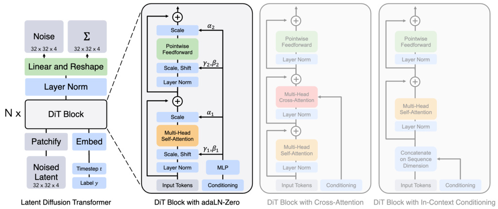
1. An image is first compressed into a smaller spatial representation (a "latent") using a pre-trained VAE
2. Take the latent representation of an input $𝑧$ as input to DiT. "Patchify" the noise latent of size $𝐼\times 𝐼\times 𝐶$ into patches of size $𝑝$ and convert it into a sequence of patches of size ${\left(\frac{𝐼}{𝑝}\right)}^2$
3. Then this sequence of tokens go through Transformer blocks. They explore three different designs for how to do generation conditioned on contextual information. Among three designs, adaLN (Adaptive layer norm)-Zero works out the best, better than in-context conditioning and cross-attention block. The scale and shift parameters, $𝛾$ and $𝛽$, are regressed from the sum of the embedding vectors of $𝑡$ and $𝑐$. The dimension-wise scaling parameters $𝛼$ is also regressed and applied immediately prior to any residual connections within the DiT block
4. The transformer decoder outputs noise predictions and an output diagonal covariance prediction

2. Scalable Interpolant Transformers (SiT)

SiT design space:

1. Time discretization: Discrete-time or continuous-time?

   • Adopting a continuous-time training framework provides significant flexibility. It decouples the model's training process from the number of steps used during sampling, which allows one to trade off inference speed and sample quality after the model is already trained.

2. Model prediction: Score or velocity field?

   • The choice of what the model predicts is critical. Training the model to predict the velocity field ($𝑣\left(𝑥,𝑡\right)$) using a velocity loss (${𝐿}_{𝑣}$), or using an equivalent weighted score loss (${𝐿}_{{𝑠}_{𝜆}}$), leads to substantially better performance than predicting the standard score. This is because the velocity parameterization effectively compensates for the vanishing gradients that the standard score objective suffers from when the noise level is low (as $𝑡\to 0$).

3. Interpolant: SBDM-VP, linear or GVP (Generalized VP)?

   • Linear (${𝛼}_{𝑡}=1-𝑡,{𝜎}_{𝑡}=𝑡$) and GVP (${𝛼}_{𝑡}=\cos \left(\frac{𝜋}{2}𝑡\right),{𝜎}_{𝑡}=\sin \left(\frac{𝜋}{2}𝑡\right)$) outperform the standard SBDM-VP path used in many diffusion models. These superior paths are more direct and have a lower "transport cost," which simplifies the learning problem by reducing the curvature of the generation trajectories.

4. Sampler: ODE or SDE? Choose which diffusion coefficient?

   • First, using a stochastic sampler (SDE) generally produces higher-quality final samples (lower FID scores) compared to a deterministic one (ODE), as it offers better theoretical control over the KL divergence.
   • Second, the diffusion coefficient (${𝑤}_{𝑡}$) in the SDE sampler is a highly effective and tunable parameter. A major finding is that ${𝑤}_{𝑡}$ can be chosen and optimized after the model has been trained, without any retraining cost. By selecting a theoretically motivated ${𝑤}_{𝑡}$ that minimizes an upper bound on the KL divergence, the model's performance can be further improved.

3. MaskDiT

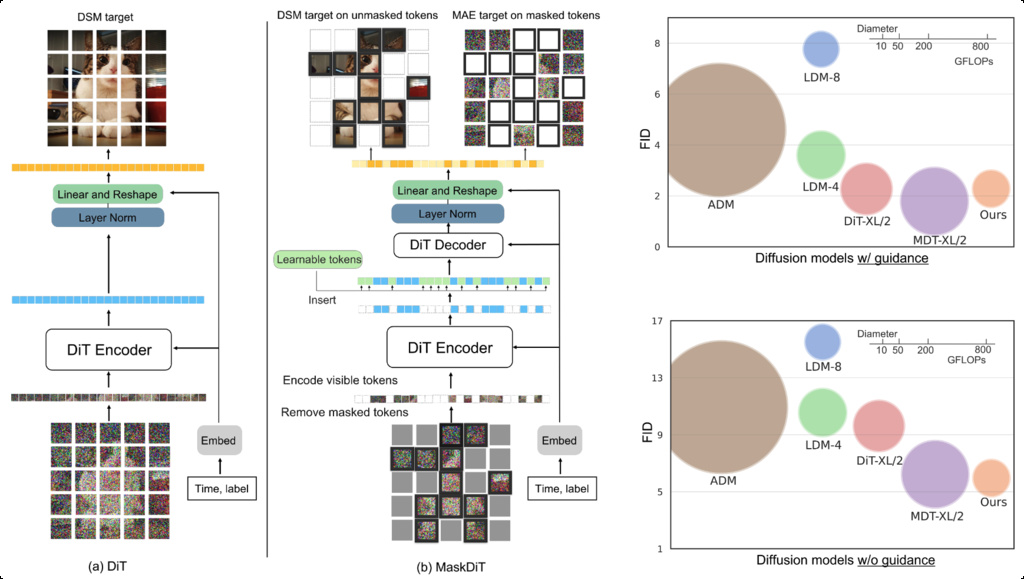
MaskDiT introduces a masked autoencoder (MAE) approach specifically designed for diffusion transformers. The key innovation lies in decomposing the traditional diffusion training objective into two complementary subtasks:

1. Score estimation on unmasked patches: The model learns to predict noise/velocity on visible image patches
2. MAE reconstruction on masked patches: The model reconstructs missing patches based on visible context

The training objective combines both tasks:

$$ℒ={ℒ}_{\text{ DSM }}+𝜆{ℒ}_{\text{ MAE}}$$

where the denoising score matching loss is:

$${ℒ}_{\text{DSM }}={𝐸}_{{𝑥}_0\sim {𝑝}_{\text{ data}}}{𝐸}_{𝑛\sim 𝑁\left(0,{𝑡}^2𝐼\right)}{𝐸}_{𝑚}{\Vert \left({𝒟}_{𝜃}\left(\left({𝑥}_0+𝑛\right)\odot \left(1-𝑚\right),𝑡\right)-{𝑥}_0\right)\odot \left(1-𝑚\right)\Vert }^2$$

and the MAE reconstruction loss is:

$${ℒ}_{\text{MAE }}={𝐸}_{{𝑥}_0\sim {𝑝}_{\text{ data}}}{𝐸}_{𝑛\sim 𝑁\left(0,{𝑡}^2𝐼\right)}{𝐸}_{𝑚}{\Vert \left({𝒟}_{𝜃}\left(\left({𝑥}_0+𝑛\right)\odot \left(1-𝑚\right),𝑡\right)-\left({𝑥}_0+𝑛\right)\right)\odot 𝑚\Vert }^2$$

Here $𝑚$ represents the binary masking pattern, $\odot$ denotes element-wise multiplication, and ${𝒟}_{𝜃}$ is the diffusion transformer model.

4. SD-DiT

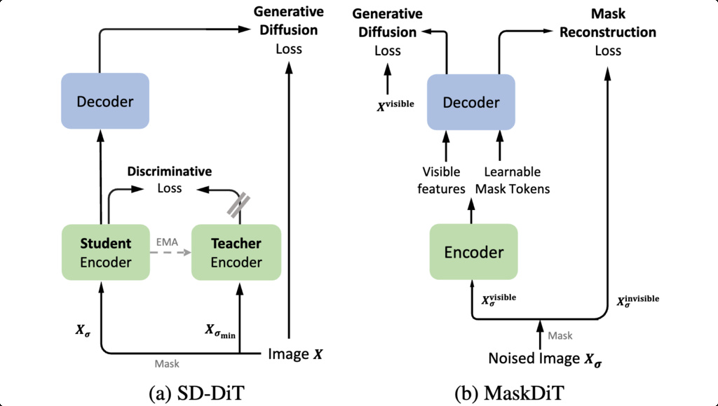
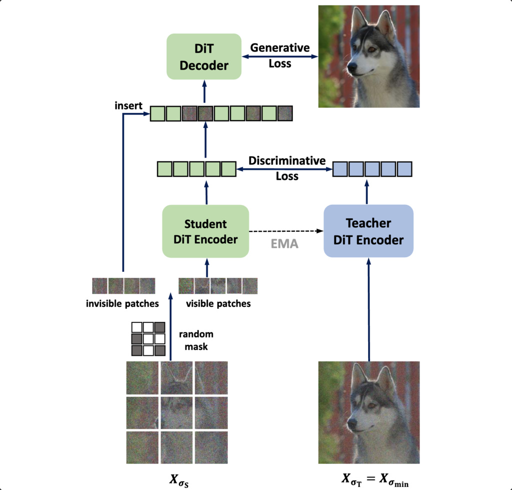
SD-DiT's architecture is built upon a decoupled encoder-decoder structure within a teacher-student scheme. This design separates the discriminative and generative learning processes. The model comprises a student encoder, a student decoder, and a teacher encoder whose weights are an exponential moving average (EMA) of the student encoder's weights.

The model is trained using two distinct objectives: a Generative Loss and a Discriminative Loss.

4.1. Generative Objective

The generative task is handled by the student branch (encoder and decoder). The student encoder processes only the visible patches of a noised and masked input image. To avoid the training-inference discrepancy, the decoder is fed the processed visible tokens along with the original, unmodified invisible patches, rather than learnable mask tokens. The objective is to denoise the full image using the standard EDM loss formulation.

The generative loss ${ℒ}_{𝐺}$ is defined as:

$${ℒ}_{𝐺}={𝐸}_{{𝑥}_0\sim {𝑝}_{\text{ data}}}{𝐸}_{𝑛\sim 𝒩\left(0,{𝜎}_{𝑆}^2𝐼\right)}{\Vert {𝐷}_{𝜃}\left({𝑥}_0+𝑛,{𝜎}_{𝑆},ℳ\right)-{𝑥}_0\Vert }_2^2$$

Here, ${𝐷}_{𝜃}$ represents the student branch, ${𝜎}_{𝑆}$ is the variable noise level for the student view, and $ℳ$ is the binary mask.

4.2. Discriminative Objective

The discriminative task aims to enforce inter-image alignment between the student and teacher encoder outputs in a shared embedding space. This is achieved by minimizing the cross-entropy loss between the softmax probability distributions of the student's visible tokens and the teacher's corresponding tokens.

The teacher view, ${𝑥}_{{𝜎}_{𝑇}}$, is created using a fixed, minimal noise level (${𝜎}_{\text{min}}$) to serve as a high-quality, stable reference, a concept inspired by Consistency Models. For each visible token $𝑖$, the loss is:

$${ℒ}_{𝐷}\left(𝑖\right)=-\sum _{𝑘}{𝑃}_{{𝑇}_{𝑖}}\log \left({𝑃}_{{𝑆}_{𝑖}}\right)$$

The total discriminative loss is averaged over all visible tokens and the [CLS] token:

$${ℒ}_{𝐷}=\frac{1}{1-ℳ}\sum _{𝑖\in \left(1-ℳ\right)}{ℒ}_{𝐷}\left(𝑖\right)+{ℒ}_{𝐷}\left(\text{[CLS]}\right)$$

The final training objective for the student network is the sum of both losses:

$${ℒ}_{\text{total }}={ℒ}_{𝐺}+{ℒ}_{𝐷}$$

References

1. What are Diffusion Models?
2. Scalable Diffusion Models with Transformers
3. SiT: Exploring Flow and Diffusion-based Generative Models with Scalable Interpolant Transformers
4. Fast Training of Diffusion Models with Masked Transformers
5. SD-DiT: Unleashing the Power of Self-supervised Discrimination in Diffusion Transformer