1. Directly model $𝑝\left(𝑥\right)$

1.1. Hopfield Network

Associative memories networks try to associate an input with its most similar pattern. The purpose is to store and retrieve patterns.

The Energy of Hopfield Network is $𝐸=-𝐷=-{\sum }_{𝑖<𝑗}{𝑤}_{𝑖𝑗}{𝑦}_{𝑖}{𝑦}_{𝑗}-{\sum }_{𝑖}{𝑏}_{𝑖}{𝑦}_{𝑖}=-\frac{1}{2}{𝑦}^{𝑇}𝑊𝑦-{𝑏}^{𝑇}𝑦$.

At each time each neuron receives a "field" ${𝑧}_{𝑖}={\sum }_{𝑗\ne 𝑖}{𝑤}_{𝑖𝑗}{𝑦}_{𝑗}+{𝑏}_{𝑖}$. If ${𝑧}_{𝑖}>0$, then ${𝑦}_{𝑖}=1$ is preferred; if ${𝑧}_{𝑖}<0$, then ${𝑦}_{𝑖}=-1$ is preferred. If everything is preferred, the $𝐷$ is maximized. If not, we have to flip some neurons to make it preferred.

Any flip that changes ${𝑦}_{𝑖}^{-}$ to ${𝑦}_{𝑖}^{+}$ increases $𝐷$ by $\mathrm{\Delta }𝐷={𝑦}_{𝑖}^{+}\left({\sum }_{𝑗\ne 𝑖}{𝑤}_{𝑖𝑗}{𝑦}_{𝑗}+{𝑏}_{𝑖}\right)-{𝑦}_{𝑖}^{-}\left({\sum }_{𝑗\ne 𝑖}{𝑤}_{𝑖𝑗}{𝑦}_{𝑗}+{𝑏}_{𝑖}\right)=2{𝑦}_{𝑖}^{+}\left({\sum }_{𝑗\ne 𝑖}{𝑤}_{𝑖𝑗}{𝑦}_{𝑗}+{𝑏}_{𝑖}\right)$. Since $𝐷\le {\sum }_{𝑖<𝑗}\left|{𝑤}_{𝑖𝑗}\right|+{\sum }_{𝑖}\left|{𝑏}_{𝑖}\right|$, we know it converges with a finite number of flips.

Training: If we want to store ${𝑁}_{𝑝}$ patterns, we use Hebbian Learning Rule to set ${𝑤}_{𝑖𝑗}\leftarrow \frac{1}{{𝑁}_{𝑝}}{\sum }_{𝑝}{𝑦}_{𝑖}^{𝑝}{𝑦}_{𝑗}^{𝑝}$ to get lowest possible energy. But this may cause spurious local optima.

How to prevent spurious local optima? We have to modify the energy landscape. We can use negative samples to do contrastive learning, which means we also maximize $𝐸$ for all non-desired patterns. $𝑊=\arg \underset{𝑊}{\min }{\sum }_{𝑦\in 𝑃}𝐸\left(𝑦\right)-{\sum }_{{𝑦}^{\prime }\notin 𝑃}𝐸\left({𝑦}^{\prime }\right)$, we can use SGD to optimize $𝑊$: ${𝑊}_{𝑡+1}={𝑊}_{𝑡}-𝜂\left({\sum }_{𝑦\in 𝑃}𝑦{𝑦}^{𝑇}-{\sum }_{{𝑦}^{\prime }\notin 𝑃}{𝑦}^{\prime }{𝑦}^{\prime 𝑇}\right)$. Since only those shallow valleys may misdirect model, we try to broaden desired patterns valleys and narrow non-desired patterns valleys. So we update $𝑊$ by ${𝑊}_{𝑡+1}={𝑊}_{𝑡}-𝜂\left({\sum }_{𝑦\in 𝑃}𝑦{𝑦}^{𝑇}-{\sum }_{{𝑦}^{\prime }\notin 𝑃\wedge {𝑦}^{\prime }\in \text{ valley}}{𝑦}^{\prime }{𝑦}^{\prime 𝑇}\right)$. We initialize ${𝑦}^{\prime }$ by all the desired patterns and run evolution for ${𝑦}^{\prime }$ with small random noise to get the valley that is close to the desired valley since those are most misleading.

But there's another problem: Naively forcing a valley to raise may hurt the learned representation. Thus we only run evolution for ${𝑦}^{\prime }$ for a few timesteps.

1.2. Boltzmann Machine

Given an energy function ${𝐸}_{𝑇}\left(𝑆\right)$, if we follow a proper physical evolution process, the system state will converge to the Boltzmann distribution ${𝑃}_{𝑇}\left(𝑆\right)=\frac{1}{𝑍}\exp \left(-\frac{{𝐸}_{𝑇}\left(𝑆\right)}{𝑘𝑇}\right)$. We can generate patterns by sampling from ${𝑃}_{𝑇}\left(𝑆\right)$, which makes a deterministic process to a probabilistic one.

$𝑃\left({𝑦}_{𝑖}=1|{𝑦}_{𝑗\ne 𝑖}\right)=\frac{{𝑒}^{-{𝐸}_{{𝑦}_{𝑖}=1}}}{{𝑒}^{-{𝐸}_{{𝑦}_{𝑖}=1}}+{𝑒}^{-{𝐸}_{{𝑦}_{𝑖}=-1}}}=\frac{1}{1+{𝑒}^{-\left({𝐸}_{{𝑦}_{𝑖}=1}-{𝐸}_{{𝑦}_{𝑖}=-1}\right)}}=\frac{1}{1+\exp \left(-2{\sum }_{𝑗}{𝑤}_{𝑖𝑗}{𝑦}_{𝑗}-2{𝑏}_{𝑖}\right)}$. Thus the network revolution becomes ${𝑦}_{𝑖}^{𝑡+1}\sim \text{ Bernoulli}\left(𝜎\left({𝑧}_{𝑖}\left(𝑡\right)\right)\right)$. Retrieval a stored pattern can be done by taking the average of final $𝑀$ samples: ${𝑦}_{𝑖}=𝐼\left[\frac{1}{𝑀}{\sum }_{𝑡=𝐿-𝑀+1}^{𝐿}{𝑦}_{𝑖}\left(𝑡\right)>0\right]$ (We can take $𝑀=1$ for simplicity).

Training: $𝑃\left(𝑦\right)=\frac{\exp \left(\frac{1}{2}{𝑦}^{𝑇}𝑊𝑦\right)}{{\sum }_{{𝑦}^{\prime }}\exp \left(\frac{1}{2}{𝑦}^{\prime 𝑇}𝑊{𝑦}^{\prime }\right)}$, log likelihood $𝐿\left(𝑊\right)=\frac{1}{{𝑁}_{𝑝}}{\sum }_{𝑦\in 𝑃}\log 𝑃\left(𝑦\right)=\frac{1}{{𝑁}_{𝑝}}{\sum }_{𝑦\in 𝑃}\frac{1}{2}{𝑦}^{𝑇}𝑊𝑦-\log {\sum }_{{𝑦}^{\prime }}\exp \left(\frac{1}{2}{𝑦}^{\prime 𝑇}𝑊{𝑦}^{\prime }\right)\left)\right)$. To maximize $𝐿\left(𝑊\right)$, we can use SGD: ${\nabla }_{{𝑤}_{𝑖𝑗}}𝐿=\frac{1}{{𝑁}_{𝑝}}{\sum }_{𝑦\in 𝑃}{𝑦}_{𝑖}{𝑦}_{𝑗}-{\sum }_{{𝑦}^{\prime }}\frac{\exp \left(\frac{1}{2}{𝑦}^{\prime 𝑇}𝑊{𝑦}^{\prime }\right)}{𝑍}{𝑦}_{𝑖}^{\prime }{𝑦}_{𝑗}^{\prime }=\frac{1}{{𝑁}_{𝑝}}{\sum }_{𝑦\in 𝑃}{𝑦}_{𝑖}{𝑦}_{𝑗}-{𝐸}_{{𝑦}^{\prime }}\left[{𝑦}_{𝑖}^{\prime }{𝑦}_{𝑗}^{\prime }\right]=\frac{1}{{𝑁}_{𝑝}}{\sum }_{𝑦\in 𝑃}{𝑦}_{𝑖}{𝑦}_{𝑗}-\frac{1}{\left|𝑆\right|}{\sum }_{{𝑦}^{\prime }\in 𝑆}{𝑦}_{𝑖}^{\prime }{𝑦}_{𝑗}^{\prime }$

We use Restricted Boltzmann Machine (RBM) for faster Gibbs sampling mixing. We have hidden neurons and visible neurons and there's no intra-layer connection. Previously we sample from every neurons and Gibbs sampling gurantees the convergence, but now we can sample from hidden neurons and visible neurons alternatively. Since there are no connections within the same layer, all neurons in the same layer can be sampled in parallel.

1.2.1. Sampling

Sampling from $𝑃\left(𝑥\right)$:

1. Inverse Transform Sampling:

If a random variable $𝑋$ has a Cumulative Distribution Function (CDF) $𝐹\left(𝑥\right)=𝑃\left(𝑋\le 𝑥\right)$. We can sample a value $𝑢$ from $𝑈\left(0,1\right)$ and set $𝑥={𝐹}^{-1}\left(𝑢\right)$. This only works if we can compute CDF and its inverse.

2. Box-Muller Transform:

This is a specialized and highly efficient method for sampling from a standard normal (Gaussian) distribution. First draw ${𝑢}_1$ and ${𝑢}_2$ from the standard uniform distribution $𝑈\left(0,1\right)$. Transform them into two independent standard normal samples: ${𝑧}_1=\sqrt{-2\ln \left({𝑢}_1\right)}\cdot \cos \left(2𝜋{𝑢}_2\right)$, ${𝑧}_2=\sqrt{-2\ln \left({𝑢}_1\right)}\cdot \sin \left(2𝜋{𝑢}_2\right)$. Then Both ${𝑧}_1$ and ${𝑧}_2$ are independent random variables sampled from the standard normal distribution $𝑁\left(0,1\right)$.

3. Importance Sampling:

We can sample from $𝑃\left(𝑥\right)$ by sampling from proposal distribution $𝑞\left(𝑥\right)$ and then weighting the samples by the ratio $\frac{𝑃\left(𝑥\right)}{𝑞\left(𝑥\right)}$.

4. MCMC:

   • Irreducibility: A Markov chain is irreducible if, for any two states $𝑖,𝑗$, there exists an integer $𝑛>0$ such that: ${𝑃}_{𝑖𝑗}^{𝑛}>0$. This means it is possible to reach any state from any other state in a finite number of steps.
   • Aperiodicity: A Markov chain is aperiodic if, for every state $𝑖$, the greatest common divisor of the set $\left\{𝑛\ge 1:{𝑃}_{𝑖𝑖}^{𝑛}>0\right\}$ is 1: $\gcd \left(𝑛\ge 1:{𝑃}_{𝑖𝑖}^{𝑛}>0\right)=1$. This ensures the chain does not get trapped in cycles.
   • Existence of Stationary Distribution: There exists a distribution $𝜋$ such that: ${𝜋}_{𝑗}={\sum }_{𝑖}{𝜋}_{𝑖}{𝑃}_{𝑖𝑗}$ or in vector notation, $𝜋=𝜋𝑃$. This $𝜋$ is called the stationary or invariant distribution.
   • Detailed Balance (Reversibility): A stronger condition than stationarity, detailed balance requires that for all states $𝑖,𝑗$: ${𝜋}_{𝑖}{𝑃}_{𝑖𝑗}={𝜋}_{𝑗}{𝑃}_{𝑗𝑖}$. If this holds, then $𝜋$ is a stationary distribution for $𝑃$.
   1. Metropolis-Hastings (M-H) Algorithm:

   For $𝑡=0,1,2,\dots$:

   • Draw a candidate ${𝑥}^{\prime }$ from a proposal distribution $𝑞\left({𝑥}^{\prime }|{𝑥}_{𝑡}\right)$.
   • Compute the acceptance ratio $𝛼\left({𝑥}^{\prime }|{𝑥}_{𝑡}\right)=\min \left(1,\frac{𝑃\left({𝑥}^{\prime }\right)\cdot 𝑞\left({𝑥}_{𝑡}|{𝑥}^{\prime }\right)}{𝑃\left({𝑥}_{𝑡}\right)\cdot 𝑞\left({𝑥}^{\prime }|{𝑥}_{𝑡}\right)}\right)$, the formula simplifies to $\min \left(1,\frac{𝑃\left({𝑥}^{\prime }\right)}{𝑃\left({𝑥}_{𝑡}\right)}\right)$ if $𝑞\left({𝑥}^{\prime }|{𝑥}_{𝑡}\right)=𝑞\left({𝑥}_{𝑡}|{𝑥}^{\prime }\right)$.

   • Draw a uniform random number $𝑢$ from $𝑈\left(0,1\right)$.

     • If $𝑢\le 𝛼\left({𝑥}^{\prime }|{𝑥}_{𝑡}\right)$, then ${𝑥}_{𝑡+1}={𝑥}^{\prime }$.
     • Otherwise, ${𝑥}_{𝑡+1}={𝑥}_{𝑡}$.
   2. Gibbs Sampling:

   A special case of the M-H algorithm that is particularly efficient for multidimensional distributions, especially when the conditional distribution of each dimension is easy to sample from.

   • Randomly initialize ${𝑥}^0=\left({𝑥}_1^0,{𝑥}_2^0,\dots ,{𝑥}_{𝑑}^0\right)$.

   • For $𝑡=0,1,2,\dots$:

     • For $𝑖=1,2,\dots ,𝑑$:

       • Sample ${𝑥}_{𝑖}^{𝑡}$ from $𝑃\left({𝑥}_{𝑖}|{𝑥}_1^{𝑡},{𝑥}_2^{𝑡},\dots ,{𝑥}_{𝑖-1}^{𝑡},{𝑥}_{𝑖+1}^{𝑡-1},\dots ,{𝑥}_{𝑑}^{𝑡-1}\right)$.

1.3. Normalizing Flows

Simplify the generation process. $𝑧\to 𝑥,𝑥=𝑓\left(𝑧\right)$

Change of Variables rule:

$$𝑝\left(𝑥\right)=𝑝\left({𝑓}^{-}1\left(𝑥\right)\right)\left|\det \left(\frac{\partial {𝑓}^{-}1\left(𝑥\right)}{\partial 𝑥}\right)\right|=\frac{𝑝\left(𝑧\right)}{\left|\det \left(\frac{\partial 𝑓\left(𝑧\right)}{\partial 𝑧}\right)\right|}$$

$𝑓={𝑓}_{𝐾}⚬\dots ⚬{𝑓}_2⚬{𝑓}_1$, $\log 𝑝\left(𝑥\right)=\log 𝑝\left({𝑓}^{-1}\left(𝑥\right)\right)+{\sum }_{𝑘=1}^{𝐾}\log \det \left(\frac{\partial {𝑓}_{𝑘}\left({𝑥}_{𝑘-1}\right)}{\partial {𝑥}_{𝑘-1}}\right)$

1.3.1. Planar Flow

$$𝑓\left(𝑧\right)=𝑧+𝑢ℎ\left({𝑤}^{𝑇}𝑧+𝑏\right)$$

where $𝜆=\left\{𝑤\in {𝑅}^{𝐷},𝑢\in {𝑅}^{𝐷},𝑏\in 𝑅\right\}$ are free parameters and $ℎ(\cdot )$ is a smooth element-wise non-linearity (e.g. tanh, ReLU, etc.).

$$\left|\det \left(\frac{\partial 𝑓}{\partial 𝑧}\right)\right|=\left|\det \left(𝐼+𝑢{ℎ}^{\prime }\left({𝑤}^{𝑇}𝑧+𝑏\right){𝑤}^{𝑇}\right)\right|=\left|1+{𝑢}^{𝑇}𝑤{ℎ}^{\prime }\left({𝑤}^{𝑇}𝑧+𝑏\right)\right|$$

The flow defined by the transformation modifies the initial density ${𝑞}_0$ by applying a series of contractions and expansions in the direction perpendicular to the hyperplane ${𝑤}^{𝑇}𝑧+𝑏=0$, hence we refer to these maps as planar flows.

However, ${𝑓}^{\prime }$ does not admit an analytical expression, and one must resort to iterative algorithms such as Newton's method to approximate it.

1.3.2. NICE (Non-linear Independent Component Estimation)

We denote $𝑧=𝑓\left(𝑥\right)$ and call $𝑓$ the encoder and its inverse ${𝑓}^{-1}$ the decoder. With ${𝑓}^{-1}$ given, we can generate $𝑥$ from $𝑧$ by ancestral sampling.

We want "easy determinant of the Jacobian" and "easy inverse".

General Coupling Layer: Partition $𝑥$ into two disjoint subsets ${𝑥}_{{𝐼}_1}$ and ${𝑥}_{{𝐼}_2}$. We can define $ℎ=\left({ℎ}_{{𝐼}_1},{ℎ}_{{𝐼}_2}\right)$, where ${ℎ}_{{𝐼}_1}={𝑥}_{{𝐼}_1},{ℎ}_{{𝐼}_2}=𝑔\left({𝑥}_{{𝐼}_2};𝑚\left({𝑥}_{{𝐼}_1}\right)\right)$, $𝑚$ is a function (e.g. MLP) and $𝑔$ is the coupling law. We consider ${𝐼}_1=\left[\left[1,𝑑\right]\right]$ and ${𝐼}_2=\left[\left[𝑑+1,𝐷\right]\right]$, then

$$\frac{\partial ℎ}{\partial 𝑥}=\left(\begin{array}{cc}{𝐼}_{𝑑}& 0\\ \frac{\partial {ℎ}_{{𝐼}_2}}{\partial {𝑥}_{{𝐼}_1}}& \frac{\partial {ℎ}_{{𝐼}_2}}{\partial {𝑥}_{{𝐼}_2}}\end{array}\right),\det \frac{\partial ℎ}{\partial 𝑥}=\det \left(\frac{\partial {ℎ}_{{𝐼}_2}}{\partial {𝑥}_{{𝐼}_2}}\right)$$

For simplicity, we choose additive coupling law $𝑔\left(𝑎;𝑏\right)=𝑎+𝑏$. Thus ${𝑥}_{{𝐼}_1}={ℎ}_{{𝐼}_1},{𝑥}_{{𝐼}_2}={ℎ}_{{𝐼}_2}-𝑚\left({ℎ}_{{𝐼}_1}\right),\det \frac{\partial ℎ}{\partial 𝑥}=1$. Each transformation is simple, so we stack multiple layers to get a complex transformation. $𝑥={ℎ}^0\leftrightarrow {ℎ}^1\leftrightarrow \dots \leftrightarrow {ℎ}^{𝐾}=𝑧,\det \frac{\partial 𝑧}{\partial 𝑥}=1$.

Combining coupling layers: Since a coupling layer leaves part of its input unchanged, we need to exchange the role of the two subsets in the partition in alternating layers, so that the composition of two coupling layers modifies every dimension.

Re-Scaling Layer: we include a diagonal scaling matrix $𝑆$ as the top layer to ensure non-unit volume transformation, which multiplies the i-th ouput value by ${𝑆}_{𝑖𝑖}$: ${\left({𝑥}_{𝑖}\right)}_{𝑖\le 𝐷}\to {\left({𝑆}_{𝑖𝑖}{𝑥}_{𝑖}\right)}_{𝑖\le 𝐷}$. This allows the learner to give more weight (i.e. model more variation) on some dimensions and less in others. In the limit where ${𝑆}_{𝑖𝑖}$ goes to $+\infty$ for some $𝑖$, the effective dimensionality of the data has been reduced by 1. We can relate these scaling factors to the eigenspectrum of a PCA, showing how much variation is present in each of the latent dimensions (the larger ${𝑆}_{𝑖𝑖}$ is, the less important the dimension $𝑖$ is).

Inpainting: For inpainting we clamp the observed dimensions (${𝑥}_{𝑂}$) to their values and maximize loglikelihood with respect to the hidden dimensions (${𝑋}_{𝐻}$) using projected gradient ascent (to keep the input in its original interval of values) with gaussian noise with step size ${𝛼}_{𝑖}=\frac{10}{100+𝑖}$ , where i is the iteration, following the stochastic gradient update:

$${𝑥}_{𝐻,𝑖+1}={𝑥}_{𝐻,𝑖}+{𝛼}_{𝑖}\left(\left(\partial \log \left({𝑝}_{𝑋}\frac{{𝑥}_{𝑂}}{\partial {𝑥}_{𝐻,𝑖}}\right),{𝑥}_{𝐻,𝑖}\right)\right)+𝜀)$$

1.3.3. Real NVP

Real-valued non-volume preserving (Real NVP) transformations.

Affine Coupling Layer: ${ℎ}_{1:𝑑}={𝑥}_{1:𝑑},{ℎ}_{𝑑+1:𝐷}={𝑥}_{𝑑+1:𝐷}\odot \exp \left(𝑠\left({𝑥}_{1:𝑑}\right)\right)+𝑡\left({𝑥}_{1:𝑑}\right)$, where $𝑠$ and $𝑡$ stand for scale and translation. The Jacobian of this transformation is

$$\frac{\partial ℎ}{\partial {𝑥}^{𝑇}}=\left(\begin{array}{cc}{𝐼}_{𝑑}& 0\\ \frac{\partial {ℎ}_{𝑑+1:𝐷}}{\partial {𝑥}_{1:𝑑}^{𝑇}}& \text{diag}\left(\exp \left(𝑠\left({𝑥}_{1:𝑑}\right)\right)\right)\end{array}\right)$$

And the inverse transformation is ${𝑥}_{1:𝑑}={ℎ}_{1:𝑑},{𝑥}_{𝑑+1:𝐷}=\left({ℎ}_{𝑑+1:𝐷}-𝑡\left({ℎ}_{1:𝑑}\right)\right)\odot \exp \left(-𝑠\left({ℎ}_{1:𝑑}\right)\right)$.

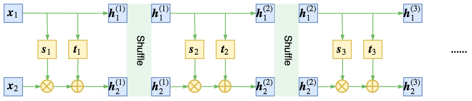
1.3.4. GLOW

NICE exchanges partitions, Real NVP shuffles, GLOW uses learnable and invertible 1x1 convolutions as mixing layers. $\log \left|\det \frac{\partial \text{ conv2D}\left(ℎ;𝑊\right)}{\partial ℎ}\right|=ℎ\cdot 𝑤\cdot \log \left|\det 𝑊\right|$. The cost of computing or differentiating $\det 𝑊$ is $𝑂\left({𝑐}^3\right)$. We use LU decomposition to reduce to $𝑂\left(𝑐\right)$. $𝑊=𝑃𝐿\left(𝑈+\text{ diag}\left(𝑠\right)\right)$, where $𝑃$ is a permutation matrix, $𝐿$ is a lower triangular matrix with ones on the diagonal, $𝑈$ is a diagonal matrix with zeros on the diagonal, and $𝑠$ is a vector. $\log \left|\det 𝑊\right|=\sum \left(\log \left|𝑠\right|\right)$.