1. Consistency Models

While diffusion models achieve remarkable sample quality, they require hundreds or thousands of function evaluations during generation, making them computationally expensive for real-time applications.

The key insight behind Consistency Models is to learn a direct mapping from noise to data, enabling single-step generation while preserving the high-quality outputs characteristic of diffusion models.

1.1. The Core Intuition

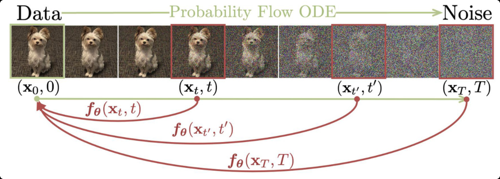
The fundamental idea of Consistency Models stems from a simple yet powerful observation: if we can learn to map any point on a diffusion trajectory directly to its corresponding clean data point, we can bypass the iterative denoising process entirely.

Consider the probability flow ODE that underlies diffusion models:

$$𝑑𝒙=\left[𝒇\left(𝒙,𝑡\right)-\frac{1}{2}{𝑔\left(𝑡\right)}^2{\nabla }_{𝒙}\log {𝑝}_{𝑡}\left(𝒙\right)\right]𝑑𝑡$$

This ODE defines a deterministic trajectory from noise ${𝒙}_{𝑇}\sim 𝒩\left(\mathrm{𝟎},𝐼\right)$ to data ${𝒙}_0\sim {𝑝}_{\text{ data}}$. A Consistency Model learns a function ${𝑓}_{𝜃}:\left({𝒙}_{𝑡},𝑡\right)\mapsto {𝒙}_0$ that maps any point $\left({𝒙}_{𝑡},𝑡\right)$ on this trajectory to the trajectory's origin ${𝒙}_0$.

1.1.1. Self-Consistency Property

The defining characteristic of Consistency Models is the self-consistency property:

Definition: A function $𝑓:\left(𝒙,𝑡\right)\mapsto 𝒙$ satisfies the self-consistency property if:

$$𝑓\left({𝒙}_{𝑡},𝑡\right)=𝑓\left({𝒙}_{{𝑡}^{\prime }},{𝑡}^{\prime }\right)\forall {𝒙}_{𝑡},{𝒙}_{{𝑡}^{\prime }}\text{ on the same ODE trajectory}$$

In other words, for any two points on the same trajectory, the consistency function should map both to the same endpoint. This ensures that:

1. $𝑓\left({𝒙}_0,0\right)={𝒙}_0$ (identity mapping at the boundary)
2. $𝑓\left({𝒙}_{𝑡},𝑡\right)={𝒙}_0$ for all $𝑡>0$ (consistent prediction)

1.2. Mathematical Framework

1.2.1. Parameterization

To ensure the boundary condition $𝑓\left({𝒙}_0,0\right)={𝒙}_0$, Consistency Models use a specific parameterization:

$${𝑓}_{𝜃}\left(𝒙,𝑡\right)=\{\begin{array}{cc}𝒙& \text{ if }𝑡=0\\ {𝐹}_{𝜃}\left(𝒙,𝑡\right)& \text{ if }𝑡>0\end{array}$$

where ${𝐹}_{𝜃}$ is a deep neural network. In practice, this is implemented as:

$${𝑓}_{𝜃}\left(𝒙,𝑡\right)={𝑐}_{\text{ skip }}\left(𝑡\right)𝒙+{𝑐}_{\text{ out }}\left(𝑡\right){𝐹}_{𝜃}\left(𝒙,𝑡\right)$$

with ${𝑐}_{\text{skip }}\left(0\right)=1$, ${𝑐}_{\text{out }}\left(0\right)=0$, ensuring the boundary condition is satisfied.

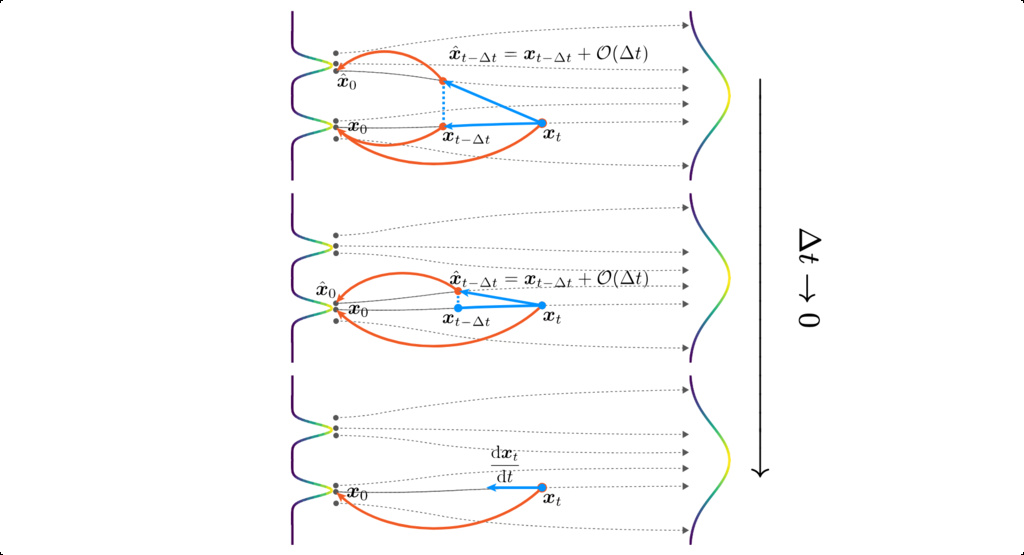
1.2.2. Discretized Training

For computational tractability, the continuous time interval $\left[0,𝑇\right]$ is discretized into $𝑁$ timesteps:

$$0={𝑡}_0<{𝑡}_1<{𝑡}_2<\dots <{𝑡}_{𝑁-1}<{𝑡}_{𝑁}=𝑇$$

The consistency function is trained to satisfy:

$${𝑓}_{𝜃}\left({𝒙}_{{𝑡}_{𝑛}},{𝑡}_{𝑛}\right)={𝑓}_{𝜃}\left({𝒙}_{{𝑡}_{𝑛+1}},{𝑡}_{𝑛+1}\right)$$

for consecutive timesteps on the same trajectory.

1.3. Training Methods

There are two primary approaches to training Consistency Models, each with distinct advantages and trade-offs.

1.3.1. Consistency Distillation (CD)

Consistency Distillation leverages a pre-trained diffusion model (teacher) to generate training pairs for the consistency model (student).

Algorithm:

1. Sample $𝒙\sim {𝑝}_{\text{ data}}$ and $𝑛\sim \text{Uniform}\left(1,𝑁-1\right)$
2. Generate noisy sample: ${𝒙}_{{𝑡}_{𝑛+1}}=𝒙+{𝑡}_{𝑛+1}𝒛$ where $𝒛\sim 𝒩\left(\mathrm{𝟎},𝐼\right)$
3. Use the pre-trained score model to estimate: ${\widehat{𝒙}}_{{𝑡}_{𝑛}}^{𝜑}={𝒙}_{{𝑡}_{𝑛+1}}+\left({𝑡}_{𝑛}-{𝑡}_{𝑛+1}\right)\mathrm{\Phi }\left({𝒙}_{{𝑡}_{𝑛+1}},{𝑡}_{𝑛+1}\right)$
4. Minimize the consistency loss:

$${ℒ}_{\text{CD }}^{𝑁}\left(𝜃,{𝜃}^{-};𝜑\right)=𝐸\left[𝜆\left({𝑡}_{𝑛}\right)𝑑\left({𝑓}_{𝜃}\left({𝒙}_{{𝑡}_{𝑛+1}},{𝑡}_{𝑛+1}\right),{𝑓}_{{𝜃}^{-}}\left({\widehat{𝒙}}_{{𝑡}_{𝑛}}^{𝜑},{𝑡}_{𝑛}\right)\right)\right]$$

where:

• $\mathrm{\Phi }$ represents the pre-trained score model parameters
• ${𝜃}^{-}$ is an exponential moving average of $𝜃$: ${𝜃}^{-}\leftarrow \text{stopgrad}\left(𝜇{𝜃}^{-}+\left(1-𝜇\right)𝜃\right)$
• $𝜆\left(𝑡\right)$ is a positive weighting function, typically $𝜆\left(𝑡\right)=1$
• $𝑑\left(·,·\right)$ is a distance metric (e.g., ${\mathrm{\ell }}_2$ or LPIPS (learned perceptual image patch similarity))

1.3.2. Consistency Training (CT)

Consistency Training learns consistency models from scratch without relying on pre-trained diffusion models.

Algorithm:

1. Sample $𝒙\sim {𝑝}_{\text{ data}}$, $𝑛\sim \text{Uniform}\left(1,𝑁-1\right)$, and $𝒛\sim 𝒩\left(\mathrm{𝟎},𝐼\right)$

2. Define adjacent points on trajectory:

   • ${𝒙}_{{𝑡}_{𝑛+1}}=𝒙+{𝑡}_{𝑛+1}𝒛$
   • ${𝒙}_{{𝑡}_{𝑛}}=𝒙+{𝑡}_{𝑛}𝒛$
3. Minimize the consistency loss:

$${ℒ}_{\text{CT }}^{𝑁}\left(𝜃,{𝜃}^{-}\right)=𝐸\left[𝜆\left({𝑡}_{𝑛}\right)𝑑\left({𝑓}_{𝜃}\left({𝒙}_{{𝑡}_{𝑛+1}},{𝑡}_{𝑛+1}\right),{𝑓}_{{𝜃}^{-}}\left({𝒙}_{{𝑡}_{𝑛}},{𝑡}_{𝑛}\right)\right)\right]$$

According to the experiments in the paper, they found,

• Heun ODE solver works better than Euler's first-order solver, since higher order ODE solvers have smaller estimation errors with the same $𝑁$.
• Among different options of the distance metric function $𝑑\left(\cdot ,\cdot \right)$, the LPIPS metric works better than ${\mathrm{\ell }}_1$ and ${\mathrm{\ell }}_2$ distance.
• Smaller $𝑁$ leads to faster convergence but worse samples, whereas larger $𝑁$ leads to slower convergence but better samples upon convergence.

1.3.3. Target Network Updates

Both training methods employ a target network ${𝑓}_{{𝜃}^{-}}$ to stabilize training. The target parameters are updated via exponential moving average:

$${𝜃}^{-}\leftarrow \text{stopgrad}\left(𝜇{𝜃}^{-}+\left(1-𝜇\right)𝜃\right)$$

where $𝜇\in \left[0,1\right)$ is the decay rate. This prevents the consistency loss from becoming degenerate (where the model simply outputs the same value for all inputs).

1.4. Sampling and Inference

1.4.1. Single-Step Sampling

The most straightforward sampling approach is single-step generation:

$${\widehat{𝒙}}_{𝜀}={𝑓}_{𝜃}\left({\widehat{𝒙}}_{𝑇},𝑇\right)\text{ where }{\widehat{𝒙}}_{𝑇}\sim 𝒩\left(\mathrm{𝟎},{𝑇}^2𝐼\right)$$

The key insight is that ${𝑓}_{𝜃}$ has learned to map any point on the diffusion trajectory back to the clean data, so we can start from pure noise and get the final result immediately.

1.4.2. Multi-Step Sampling

While single-step sampling is fast, multi-step sampling can improve quality by alternating denoising and noise injection steps:

This process allows trading computational cost for sample quality, similar to how diffusion models work but with far fewer steps.

1.5. Improved Consistency Training (iCT)

1. Removing EMA for the Teacher Network: The authors identified a theoretical flaw where using Exponential Moving Average (EMA) for the teacher network provides no useful training signal for the data distribution. By setting the EMA decay rate to zero ($𝜇\left(𝑘\right)=0$), they ensure the teacher and student parameters are correctly aligned, which significantly boosts performance.
2. Pseudo-Huber Loss: To replace the biased and computationally expensive LPIPS metric, the authors adopt the Pseudo-Huber loss, defined as $𝑑\left(𝑥,𝑦\right)=\sqrt{{\Vert 𝑥-𝑦\Vert }_2^2+{𝑐}^2}-𝑐$. This simple metric is robust to outliers, reduces training variance, and ultimately surpasses the performance of LPIPS-based training.
3. Improved Discretization Curriculum: The paper demonstrates that model performance scales with the number of discretization steps ($𝑁$) according to a power law. Based on this, they propose a new exponential curriculum for $𝑁\left(𝑘\right)$—doubling $𝑁$ at fixed intervals—which empirically yields the best sample quality.
4. Lognormal Noise Schedule: The default training procedure over-emphasizes high noise levels. The authors introduce a lognormal noise schedule to focus training on more critical low-to-mid noise ranges, leading to a notable improvement in sample quality.
5. Optimized Hyperparameters: The work also introduces an improved weighting function ($𝜆\left({𝜎}_{𝑖}\right)=\frac{1}{{𝜎}_{𝑖+1}-{𝜎}_{𝑖}}$), increased dropout rates, and fine-tuned noise embeddings to further enhance performance.

1.6. Simplifying, Stabilizing and Scaling Continuous-Time Consistency Models (sCM)

• Discrete-time CMs The training objective is defined at two adjacent time steps with finite distance:

  $${𝐸}_{{𝒙}_{𝑡},𝑡}\left[𝑤\left(𝑡\right)𝑑\left({𝑓}_{𝜃}\left({𝒙}_{𝑡},𝑡\right),{𝑓}_{{𝜃}^{-}}\left({𝒙}_{𝑡-\mathrm{\Delta }𝑡},𝑡-\mathrm{\Delta }𝑡\right)\right)\right]$$

  where ${𝜃}^{-}$ denotes $\text{stopgrad}\left(𝜃\right)$, $𝑤\left(𝑡\right)$ is the weighting function, $\mathrm{\Delta }𝑡>0$ is the distance between two adjacent time steps, and $𝑑\left(\cdot ,\cdot \right)$ is the distance metric.

• Continuous-time CMs We use $𝑑\left(𝑥,𝑦\right)={\Vert 𝑥-𝑡\Vert }^2$ and take $\mathrm{\Delta }𝑡\to 0$, we can show that

  $$\underset{\mathrm{\Delta }𝑡\to 0}{\lim }{𝐸}_{{𝒙}_{𝑡},𝑡}\left[𝑤\left(𝑡\right)𝑑\left({𝑓}_{𝜃}\left({𝒙}_{𝑡},𝑡\right),{𝑓}_{{𝜃}^{-}}\left({𝒙}_{𝑡-\mathrm{\Delta }𝑡},𝑡-\mathrm{\Delta }𝑡\right)\right)\right]={\nabla }_{𝜃}{𝐸}_{{𝒙}_{𝑡},𝑡}\left[𝑤\left(𝑡\right){𝑓}_{𝜃}^{𝑇}\left({𝒙}_{𝑡},𝑡\right)\frac{𝑑{𝑓}_{{𝜃}^{-}}\left({𝒙}_{𝑡},𝑡\right)}{𝑑𝑡}\right]$$

  where $\frac{𝑑{𝑓}_{{𝜃}^{-}}\left({𝒙}_{𝑡},𝑡\right)}{𝑑𝑡}={\nabla }_{{𝒙}_{𝑡}}{𝑓}_{{𝜃}^{-}}\left({𝒙}_{𝑡},𝑡\right)\frac{𝑑{𝒙}_{𝑡}}{𝑑𝑡}+{\partial }_{𝑡}{𝑓}_{{𝜃}^{-}}\left({𝒙}_{𝑡},𝑡\right)$ is the tangent of ${𝑓}_{{𝜃}^{-}}$ at $\left({𝒙}_{𝑡},𝑡\right)$ along the trajectory of the PF-ODE $\frac{𝑑𝒙}{𝑑𝑡}$.

  Notably, continuous-time CMs do not rely on ODE solvers, which avoids discretization errors and offers more accurate supervision signals during training. However, previous work found that training continuous-time CMs, or even discrete-time CMs with an extremely small $\mathrm{\Delta }𝑡$, suffers from severe instability in optimization. This greatly limits the empirical performance and adoption of continuous-time CMs.

To address the stability issues of continuous-time consistency models, researchers introduced TrigFlow - a simplified theoretical framework that unifies EDM (Elucidated Diffusion Models) and Flow Matching while significantly simplifying the mathematical formulation.

TrigFlow uses trigonometric functions to parameterize the diffusion process, making the mathematical expressions much cleaner and more stable. The key insight is to replace the complex EDM coefficients with simple trigonometric functions:

Diffusion Process:

$${𝒙}_{𝑡}=\cos \left(𝑡\right){𝒙}_0+\sin \left(𝑡\right)𝒛$$

where $𝑡\in \left[0,\frac{𝜋}{2}\right]$ and $𝒛\sim 𝒩\left(\mathrm{𝟎},{𝜎}_{𝑑}^2𝑰\right)$.

Diffusion Models and PF-ODE:

$${𝑓}_{𝜃}^{\text{DM }}\left({𝒙}_{𝑡},𝑡\right)={𝐹}_{𝜃}\left(\frac{{𝒙}_{𝑡}}{{𝜎}_{𝑑}},{𝑐}_{\text{ noise }}\left(𝑡\right)\right)$$

where ${𝐹}_{𝜃}$ is a neural network with parameters $𝜃$, and ${𝑐}_{\text{noise }}\left(𝑡\right)$ is a transformation of $𝑡$ to facilitate time conditioning. The corresponding PF-ODE is given by

$$\frac{𝑑{𝒙}_{𝑡}}{𝑑𝑡}={𝜎}_{𝑑}{𝐹}_{𝜃}\left(\frac{{𝒙}_{𝑡}}{{𝜎}_{𝑑}},{𝑐}_{\text{ noise }}\left(𝑡\right)\right)$$

Training Target:

$${ℒ}_{\text{Diff }}\left(𝜃\right)={𝐸}_{{𝑥}_0,𝑧,𝑡}\left[{\Vert {𝜎}_{𝑑}{𝐹}_{𝜃}\left(\frac{{𝒙}_{𝑡}}{{𝜎}_{𝑑}},{𝑐}_{\text{ noise }}\left(𝑡\right)\right)-{𝑣}_{𝑡}\Vert }_2^2\right]$$$${𝒗}_{𝑡}=\cos \left(𝑡\right)𝒛-\sin \left(𝑡\right){𝒙}_0$$

Consistency Model Parameterization:

$$\begin{array}{c}{𝑐}_{\text{skip }}\left(𝑡\right)=\cos \left(𝑡\right),{𝑐}_{\text{ out }}\left(𝑡\right)=-{𝜎}_{𝑑}\sin \left(𝑡\right),{𝑐}_{\text{ in }}\left(𝑡\right)=\frac{1}{{𝜎}_{𝑑}}\\ {𝑓}_{𝜃}\left({𝒙}_{𝑡},𝑡\right)=\cos \left(𝑡\right){𝒙}_{𝑡}-\sin \left(𝑡\right){𝜎}_{𝑑}{𝐹}_{𝜃}\left(\frac{{𝒙}_{𝑡}}{{𝜎}_{𝑑}},{𝑐}_{\text{noise}\left(𝑡\right)}\right)\end{array}$$

1.6.1. Stabilization Techniques

The TrigFlow framework incorporates several key stabilization techniques:

• Identity Time Transformation: Using ${𝑐}_{\text{noise }}\left(𝑡\right)=𝑡$ instead of the complex logarithmic transformation from EDM prevents numerical blow-up as $𝑡\to \frac{𝜋}{2}$.
• Positional Time Embeddings: Avoiding high-frequency Fourier embeddings in favor of positional embeddings reduces gradient instability.
• Adaptive Double Normalization: Modifying the AdaGN layers to use pixel normalization for both scale and bias terms improves training stability.
• Tangent Normalization: Explicitly normalizing the tangent function $\frac{𝑑{𝑓}_{{𝜃}^{-}}\left({𝒙}_{𝑡},𝑑𝑡\right)}{𝑑𝑡}$ to control gradient variance.

1.6.2. Training Objective

To make the training objective more stable, we modify the training objective to:

$${ℒ}_{\text{sCM }}\left(𝜃,𝜑\right)={𝐸}_{{𝒙}_{𝑡},𝑡}\left[\frac{{𝑒}^{{𝑤}_{𝜑}\left(𝑡\right)}}{𝐷}{\Vert {𝐹}_{𝜃}\left(\frac{{𝒙}_{𝑡}}{{𝜎}_{𝑑}},𝑡\right)-{𝐹}_{{𝜃}^{-}}\left(\frac{{𝒙}_{𝑡}}{{𝜎}_{𝑑}},𝑡\right)-\cos \left(𝑡\right)\frac{𝑑{𝑓}_{{𝜃}^{-}}\left({𝒙}_{𝑡},𝑡\right)}{𝑑𝑡}\Vert }_2^2-{𝑤}_{𝜑}\left(𝑡\right)\right]$$

where ${𝑤}_{𝜑}\left(𝑡\right)$ is an adaptive weighting function that balances the loss across different time steps.

1.7. Consistency Trajectory Models

$$\frac{𝑑{𝒙}_{𝑡}}{𝑑𝑡}=-𝑡{\nabla }_{{𝒙}_{𝑡}}\log {𝑝}_{𝑡}\left({𝒙}_{𝑡}\right)=\frac{{𝒙}_{𝑡}-{𝐸}_{{𝑝}_{𝑡0}\left({𝒙}_0|{𝒙}_{𝑡}\right)}\left[𝒙|{𝒙}_{𝑡}\right]}{𝑡}$$

where ${𝑝}_{𝑡0}\left(𝒙|{𝒙}_{𝑡}\right)$ is the probability distribution of the solution of the reverse-time stochastic process from time $𝑡$ to zero, initiated from ${𝒙}_{𝑡}$. Here, ${𝐸}_{{𝑝}_{𝑡0}\left({𝒙}_0|{𝒙}_{𝑡}\right)}\left[𝒙|{𝒙}_{𝑡}\right]={𝒙}_{𝑡}+𝑡\nabla \log {𝑝}_{𝑡}\left({𝒙}_{𝑡}\right)$ is the denoiser function (Tweedie's Formula), an alternative expression for the score function $\nabla \log {𝑝}_{𝑡}\left({𝒙}_{𝒕}\right)$. In practice, the denoiser ${𝐸}_{{𝑝}_{𝑡0}\left({𝒙}_0|{𝒙}_{𝑡}\right)}\left[𝒙|{𝒙}_{𝑡}\right]$ is approximated using a neural network ${𝐷}_{𝜑}$, obtained by minimizing the DSM loss ${𝐸}_{{𝒙}_0,𝑡,{𝑝}_{0𝑡}\left(𝒙|{𝒙}_0\right)}\left[{\Vert {𝒙}_0-{𝐷}_{𝜑}\left({𝒙}_{𝑡},𝑡\right)\Vert }_2^2\right]$.

Sampling from DM involves solving the PF ODE, equivalent to computing the integral

$${\int }_{𝑇}^0\frac{𝑑{𝒙}_{𝑡}}{𝑑𝑡}𝑑𝑡={\int }_{𝑇}^0\frac{{𝒙}_{𝑡}-{𝐷}_{𝜑}\left({𝒙}_{𝑡},𝑡\right)}{𝑡}𝑑𝑡\iff {𝒙}_0={𝒙}_{𝑇}+{\int }_{𝑇}^0\frac{{𝒙}_{𝑡}-{𝐷}_{𝜑}\left({𝒙}_{𝑡},𝑡\right)}{𝑡}𝑑𝑡$$

where ${𝒙}_{𝑇}$ is sampled from a prior distribution $𝜋$ approximating ${𝑝}_{𝑇}$. Decoding strategies of DM primarily fall into two categories: score-based sampling with time-discretized numerical integral solvers, and distillation sampling where a neural network directly estimates the integral.

• Score-based Sampling: Despite recent advancements in numerical solvers, further improvements may be challenging due to the inherent discretization error present in all solvers, ultimately limiting the sample quality obtained with few NFEs.
• Distillation Sampling: Distillation models' multistep sampling approach exhibits degrading sample quality with increasing NFE, lacking a clear trade-off between computational budget (NFE) and sample fidelity. Furthermore, multistep sampling is not deterministic, leading to uncontrollable sample variance.

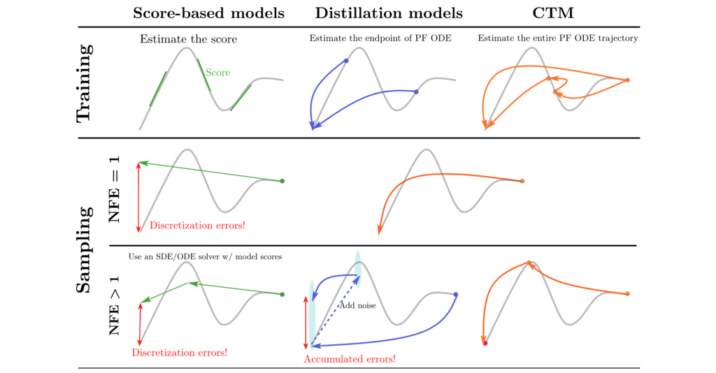
1.7.1. Trajectory Mapping Function

CTM learns a trajectory mapping function ${𝐺}_{𝜃}:\left({𝒙}_{𝑡},𝑡,𝑠\right)\mapsto {𝒙}_{𝑠}$ that maps a point ${𝒙}_{𝑡}$ at time $𝑡$ to the corresponding point ${𝒙}_{𝑠}$ at time $𝑠$ along the same ODE trajectory.

Key properties:

1. Consistency: ${𝐺}_{𝜃}\left({𝒙}_{𝑡},𝑡,𝑡\right)={𝒙}_{𝑡}$ (identity mapping)
2. Transitivity: ${𝐺}_{𝜃}\left({𝒙}_{𝑡},𝑡,𝑠\right)={𝐺}_{𝜃}\left({𝐺}_{𝜃}\left({𝒙}_{𝑡},𝑡,𝑟\right),𝑟,𝑠\right)$ for any intermediate time $𝑟$
3. Boundary condition: ${𝐺}_{𝜃}\left({𝒙}_0,0,𝑠\right)={𝒙}_{𝑠}$ where ${𝒙}_{𝑠}$ follows the forward process

For stable training, we express $𝐺$ as a mixture of ${𝒙}_{𝑡}$ and a function $𝑔$ (inspired from the Euler solver):

$$𝐺\left({𝒙}_{𝑡},𝑡,𝑠\right)=\frac{𝑠}{𝑡}{𝒙}_{𝑡}+\left(1-\frac{𝑠}{𝑡}\right)𝑔\left({𝒙}_{𝑡},𝑡,𝑠\right)$$

where $𝑔\left({𝒙}_{𝑡},𝑡,𝑠\right)={𝒙}_{𝑡}+\frac{𝑡}{𝑡-𝑠}{\int }_{𝑡}^{𝑠}\frac{{𝒙}_{𝑢}-𝐸\left[𝑥|{𝑥}_{𝑢}\right]}{𝑢}𝑑𝑢$ and we approximate $𝑔$ using ${𝑔}_{𝜃}$ with a neural network. A critical insight is that this parameterization also allows access to the score function. By taking the limit as $𝑠$ approaches $𝑡$, we find:

$$\underset{𝑠\to 𝑡}{\lim }𝑔\left({𝒙}_{𝑡},𝑡,𝑠\right)=𝐸\left[𝒙|{𝒙}_{𝑡}\right]$$

This means that CTM not only learns to make long jumps along the trajectory but also learns the infinitesimal jumps, i.e., the denoiser/score function. This property unifies score-based and distillation approaches within a single model.

1.7.2. CTM Training

CTM training combines a distillation loss with powerful auxiliary losses that provide direct training signals from the data, allowing the student (CTM) to surpass the teacher (diffusion model).

• Soft Consistency Loss: The primary loss is a distillation loss where the CTM's jump prediction ${𝐺}_{𝜃}\left({𝒙}_{𝑡},𝑡,𝑠\right)$ is matched against a target generated by a pre-trained teacher model. To make this efficient and effective, CTM uses soft consistency matching. The model is trained to enforce ${𝐺}_{𝜃}\left({𝒙}_{𝑡},𝑡,𝑠\right)\approx {𝐺}_{\text{sg}\left(𝜃\right)}\left(\text{Solver}\left({𝒙}_{𝑡},𝑡,𝑢;𝜑\right),𝑢,𝑠\right)$, where $𝑢$ is a random time between $𝑠$ and $𝑡$. This serves as a flexible interpolation between local consistency ($𝑢=𝑡-\mathrm{\Delta }𝑡$, distilling a single step) and global consistency ($𝑢=𝑠$, distilling the entire interval).

• Auxiliary Losses:

  1. Denoising Score Matching (DSM) Loss: Since CTM can estimate the denoiser via ${𝑔}_{𝜃}\left({𝒙}_{𝑡},𝑡,𝑡\right)$, it is explicitly trained with a DSM loss: ${ℒ}_{\text{DSM }}\left(𝜃\right)=𝐸\left[{\Vert {𝒙}_0-{𝑔}_{𝜃}\left({𝒙}_{𝑡},𝑡,𝑡\right)\Vert }_2^2\right]$. This regularizes the model to accurately learn the score function, which is vital for precision and for enabling score-based sampling methods.
  2. Adversarial (GAN) Loss: To further enhance sample quality and refine details, an adversarial loss ${ℒ}_{\text{GAN}}$ is added, similar to VQGAN.

The final loss is a weighted sum: $ℒ≔{ℒ}_{\text{ CTM }}+{𝜆}_{\text{ DSM }}{ℒ}_{\text{ DSM }}+{𝜆}_{\text{ GAN }}{ℒ}_{\text{ GAN}}$.

1.7.3. $𝛾$-Sampling

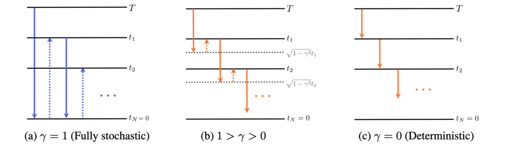
CTM's ability to travel between any two points in time enables a novel and flexible sampling scheme called $𝛾$-sampling, controlled by a parameter $𝛾\in \left[0,1\right]$. A sampling step from ${𝑡}_{𝑛}$ to ${𝑡}_{𝑛+1}$ involves:

1. Denoise: Jump from ${𝒙}_{{𝑡}_{𝑛}}$ to an intermediate time $\sqrt{1-{𝛾}^2}{𝑡}_{𝑛+1}$ using the learned function ${𝐺}_{𝜃}$.
2. Noisify: Add a controlled amount of noise to reach the noise level corresponding to time ${𝑡}_{𝑛+1}$.

This process offers a spectrum of sampling behaviors:

• $𝛾=0$ (Deterministic): The process is fully deterministic. It follows the PF ODE path directly, avoiding the discretization errors of traditional ODE solvers and the error accumulation of CM's multistep method. Sample quality consistently improves with more NFEs.
• $𝛾=1$ (Fully Stochastic): This recovers the multistep sampling method used in Consistency Models. However, this approach suffers from error accumulation, and sample quality can degrade as NFE increases.
• $0<𝛾<1$ (Hybrid): This provides a tuneable level of stochasticity, generalizing the stochastic samplers found in models like EDM.

1.8. Flow-Anchored Consistency Model (FACM)

Continuous-time Consistency Models (CMs) promise efficient few-step generation but face significant challenges with training instability. We argue this instability stems from a fundamental conflict: by training a network to learn only a shortcut across a probability flow, the model loses its grasp on the instantaneous velocity field that defines the flow.

1.8.1. The Source of Instability: Losing the Flow Anchor

The practical implementation of the continuous-time CM objective via the training target $𝑇=𝑣+\left(1-𝑡\right)\frac{𝑑{𝐹}_{{𝜃}^{-}}\left({𝒙}_{𝑡},𝑡\right)}{𝑑𝑡}$ is notoriously unstable. The core of this instability lies in the target's self-referential nature, creating two fundamental, intertwined problems:

1. Missing Instantaneous Velocity Field Supervision: The target $𝑇$ explicitly depends on the ground-truth instantaneous velocity $𝑣$. The CM objective, however, only enforces a loss on the final prediction ${𝐹}_{𝜃}$ (the average velocity). There is no explicit mechanism to ensure that the model's learned dynamics remains faithful to the underlying instantaneous velocity field $𝑣$.

2. Self-Referential Derivative Estimation: The network is required to estimate its own derivative. Even if the network is pre-trained and initially provides a good approximation of the instantaneous velocity, the CM objective alone provides no continuous supervision to maintain this alignment.

1.8.2. Flow-Anchoring Principle

Stability can be achieved by explicitly anchoring the model in the very flow it is shortcutting. The most direct way to achieve this Flow-Anchoring is to re-introduce the explicit training of the instantaneous velocity field that defines the flow.

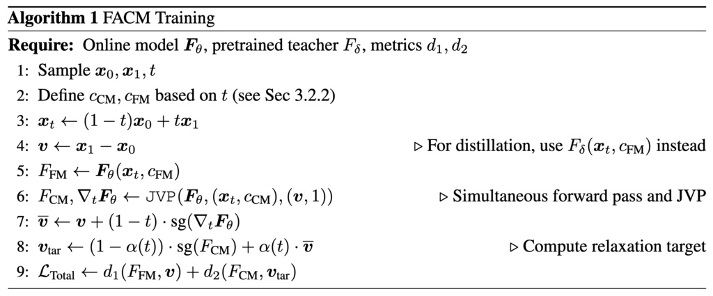
1.8.3. FACM Training Strategy

FACM employs a simple yet effective training strategy that mixes two complementary objectives:

$${ℒ}_{\text{FACM }}={ℒ}_{\text{ FM }}+{ℒ}_{\text{ CM}}$$

1.8.3.1. Flow Matching Loss (The Anchor)

This loss component anchors the model by regressing its output towards the instantaneous velocity $𝑣$:

$${ℒ}_{\text{FM }}\left(𝜃\right)=𝐸\left[{\Vert {𝐹}_{𝜃}\left({𝒙}_{𝑡},{𝑐}_{\text{ FM}}\right)-𝑣\Vert }_2^2+{ℒ}_{\text{ cos }}\left({𝐹}_{𝜃}\left({𝒙}_{𝑡},{𝑐}_{\text{ FM}}\right),𝑣\right)\right]$$

where ${ℒ}_{\text{cos }}\left(𝑎,𝑏\right)=1-\frac{𝑎\cdot 𝑏}{{\Vert 𝑎\Vert }_2{\Vert 𝑏\Vert }_2}$

1.8.3.2. Consistency Model Loss (The Accelerator)

This component acts as an accelerator, training the model to learn the generative shortcut. We interpret the consistency condition as a fixed-point problem:

$${𝐹}_{𝜃}=𝑇\left({𝐹}_{𝜃}\right),\text{ where }𝑇\left(𝐹\right)=𝑣+\left(1-𝑡\right)\frac{𝑑𝐹}{𝑑𝑡}$$

First, we compute the consistency residual $𝑔$ of the stop-gradient model ${𝐹}_{{𝜃}^{-}}$:

$$𝑔={𝐹}_{{𝜃}^{-}}\left({𝒙}_{𝑡},{𝑐}_{\text{ CM}}\right)-𝑇\left({𝐹}_{{𝜃}^{-}}\right)$$

Then form a perturbed target:

$${𝑣}_{\text{tar }}={𝐹}_{{𝜃}^{-}}\left({𝒙}_{𝑡},{𝑐}_{\text{ CM}}\right)-𝛼\left(𝑡\right)\cdot 𝑔=\left(1-𝛼\left(𝑡\right)\right){𝐹}_{{𝜃}^{-}}\left({𝒙}_{𝑡},{𝑐}_{\text{ CM}}\right)+𝛼\left(𝑡\right)𝑇\left({𝐹}_{{𝜃}^{-}}\right)$$

This formulation provides a stable, interpolated learning target between the current model's output and the ideal consistency target. The final CM loss component uses a norm L2 loss, ${𝐿}_{\text{norm}}$, and is modulated by weighting functions $𝛼\left(𝑡\right)$ and $𝛽\left(𝑡\right)$:

$${ℒ}_{\text{CM }}\left(𝜃\right)=𝐸\left[𝛽\left(𝑡\right)\cdot {𝐿}_{\text{ norm }}\left({𝐹}_{𝜃}\left({𝑥}_{𝑡},{𝑐}_{\text{ CM}}\right),{𝑣}_{\text{ tar}}\right)\right]$$

It is important to note that our specific choices for weighting and loss functions are designed to accelerate convergence, not as prerequisites for stability, which is guaranteed by the Flow-Anchoring principle.

1.8.4. Implementation of the Mixed Objective

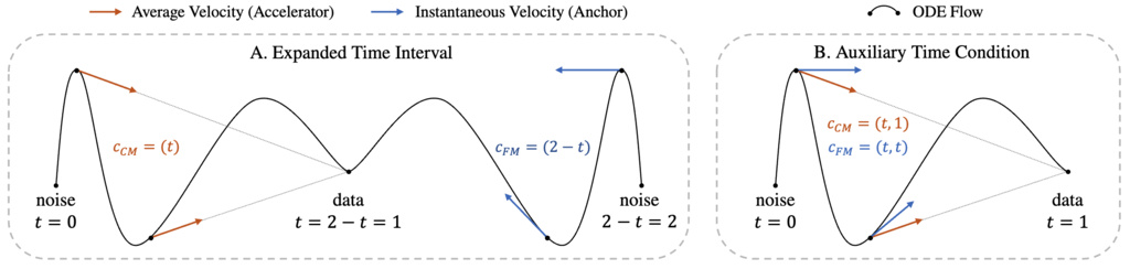
1.8.4.1. Expanded Time Interval Strategy

We innovatively propose leveraging an expanded time domain to distinguish between the two tasks:

• CM Task: Operates on the interval $𝑡\in \left[0,1\right]$, using ${𝑐}_{\text{CM }}=𝑡$
• FM Task: Maps to the alternate interval $\left[1,2\right]$ by setting ${𝑐}_{\text{FM }}=2-𝑡$

This mapping ensures continuity at the boundary $𝑡=1$:

$$\underset{𝑡\to 1^{-}}{\lim }\left[𝑣+\left(1-𝑡\right)\frac{𝑑{𝐹}_{𝜃}\left({𝒙}_{𝑡},𝑡\right)}{𝑑𝑡}\right]=𝑣$$

1.8.4.2. Auxiliary Condition Strategy

Alternatively, we can introduce a second time variable $𝑟$, making the model's full conditioning a tuple of $\left(𝑡,𝑟\right)$:

• ${𝑐}_{\text{CM }}=\left(𝑡,1\right)$: Model learns CM task (average velocity from $𝑡$ to $1$)
• ${𝑐}_{\text{FM }}=\left(𝑡,𝑡\right)$: Model learns FM task (instantaneous velocity at $𝑡$)

References

1. Consistency Models
2. What are Diffusion Models?
3. Improved Techniques for Training Consistency Models
4. Simplifying, Stabilizing and Scaling Continuous-Time Consistency Models
5. Consistency Trajectory Models: Learning Probability Flow ODE Trajectory of Diffusion
6. Flow-Anchored Consistency Model